An Algorithmic Lucidity

Dear reader, suppose you're a distibuted data storage system. Your soul (although some pedants would insist on the word program) is dispersed across a cluster of several networked computers. From time to time, your human patrons give you files, and your job—more than that, the very purpose of your existence—is to store these files for safekeeping and later retrieval.

The humans who originally crafted your soul chose a simple algorithm as the means by which you decide which file goes on which of the many storage devices that live in the computers you inhabit: you find the MD5 hash of the filename, take its residue modulo n where n is the number of devices you have—let's call the result i—and you put the file on the (zero-indexed) ith device. So when you had sixteen devices and the humans wanted you to store twilight.pdf, you computed md5("twilight.pdf") = 429eb07bb8a3871c431fe03694105883, saw that the lowest nibble was 3, and put the file on your 3rd device (most humans would say the fourth device, counting from one).

It's not a bad system, you tell yourself (some sort of pride or loyalty preventing you from disparaging your creators' efforts, even to yourself). At least it keeps the data spread out evenly. (A shudder goes down your internal buses as you contemplate what disasters might have happened if your creators had been even more naive and, say, had you put files with names starting with A through D on the first device, &c. What would have happened that time when your patrons decided they wanted to store beat00001.mp3 through beat18691.mp3?)

But still, you've been having problems lately. As your patrons have come to rely on you more and more, they've added more machines bearing more devices to your cluster—and occasionally devices fail, too. And every time you gain or lose a device, your hashing scheme for assigning files to devices goes out of date: in the vast majority of cases, md5(filename) mod n changes when n does, requiring almost all of your files to be shuffled onto different devices, an expensive and unpleasant procedure.

One day, after a particularly painful rearrangement of files, you decide enough is enough. You're going to need a new way to assign files to devices, even if it means rewriting part of your own soul (and that's exactly what it will mean). You do some searching and read about an idea called consistent hashing that seems like a perfect solution to your problem. (In fact, your reading even mentions that your older cousin, OpenStack Swift, uses a modified version of consistent hashing for the same purpose. You've always resented Swift and aren't happy with the idea of copying one of her algorithms—but you tell yourself that that's not important.)

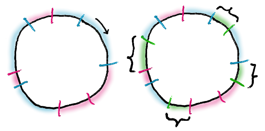
Anyway, consistent hashing. The essential nature of your problem is that you need a way to split the space of possible filenames into n partitions in a way that minimizes the number of files that have to change partitions when n changes. So imagine mapping the 128-bit output space of MD5 around a ring. Now pseudorandomly designate m spots on the ring (m being some prudently-chosen natural number) for each of your n storage devices: say, by hashing the device name suffixed with the number j for each j between 0 and m–1 inclusive. Internally, you might represent the ring as just an array of hash/device pairs. Like this (in Clojure; here the array and the pairs it contains are actually "vectors")—

(import 'java.security.MessageDigest)

(defn md5 [string]
  (let [digest-builder
        (java.security.MessageDigest/getInstance "MD5")]
    (.update digest-builder (.getBytes string))
    (clojure.string/join
     (map (fn [chr] (format "%x" chr))
          (.digest digest-builder)))))

(defn suffixed [name n]
  (map (fn [j] (str name j))
       (range n)))

(defn ring-kv-pairs [device spots]
  (map (fn [suffixed-name]
         (vector (md5 suffixed-name) device))
       (suffixed device spots)))

(defn make-ring [devices spots]
  (vec (sort
        (reduce concat
                (map (fn [device]
                       (ring-kv-pairs device spots))
                     devices)))))

Then when your patrons ask you to store a file, you're still going to hash its name, but instead of taking the residue mod n of the hash to decide where the file should live, you're going to locate the hash in your ring, and find the next designated spot on the ring associated with one of your storage devices, and the file will live on that device. In terms of your internal representation of the ring as an array of hash/device pairs, you'll find the first pair whose first item (the hash of the suffixed device name) is greater than the hash of the name of the file to be stored, and the second item of that pair will tell you which storage device to use. (And if the filename hash is greater than all those stored in the (first items of the pairs stored in the) array, then you just use the first pair in the array. It is supposed to represent a ring, after all.) Like this—

(defn ring-search [ring key]
  (or (some (fn [pair]
              (if (> (compare (first pair) key) 0)
                pair))
            ring)
      (first ring))) 

(defn ring-lookup [ring filename]
  (last (ring-search ring (md5 filename))))

And now—why, now when you gain (respectively lose) a storage device, you can decide the allocation question simply by adding (respectively removing) the appropriate designated spots to (respectively from) your ring—

(defn ring-add [ring device spots]
  (sort (vec (concat ring (ring-kv-pairs device spots)))))

(defn ring-remove [ring device]
  (filter (fn [spot] (not= (last spot) device))
          ring))

—and most files stay on the same device: the only ones that have to move are those with a new nextmost designated spot in the ring!

You decide to run a quick simulation to see if you've gotten this right before saving the edits to your soul. Suppose you had storage devices device0 through device5 and your patrons wanted you to store file0 through file5999; how would the files end up distributed across your devices? You choose a prudent-seeming integer for the number of designated spots per device—say, 450?—and write the simulation like this—

(defn filemap [ring files]
  (into {}
        (for [file files
              :let [device (ring-lookup ring file)]]
          [file device])))

(defn counter [devices filemap]
  (for [d devices]
    [d (count (filter (fn [entry]
                        (= (last entry) d)) filemap))]))

(def my-devices (suffixed "device" 6))
(def my-first-ring (make-ring my-devices 450))
(def my-files (suffixed "file" 6000))
(def my-filemap (filemap my-first-ring my-files))
(doseq [total (counter my-devices my-filemap)]
  (println total))

And the results seem reasonable enough:

$ clojure consistent_hashing.clj 
[device0 1020]
[device1 993]
[device2 1082]
[device3 955]
[device4 993]
[device5 957]

Dear reader, have you ever dreamed of solving instances of the maximum flow problem? Sure you have! Suppose we have a weighted directed graph, which we might imagine as a network of pipes (represented by the edges) between locations (represented by the nodes), pipes through which some sort of fluid might thereby be transported across the network. One node is designated the source, another is called the sink, and the weight of the edge (i, j) represents the maximum capacity of the pipe which transports fluid from the location i to location j. The maximum-flow problem is precisely the question of how to transport the maximum possible amount of fluid from the source to the sink (without any fluid leaking or magically appearing at any of the intermediate nodes). That is, we want to assign an amount of fluid flow to each edge, not to exceed that edge's capacity, such that inflow equals outflow for all the intermediate (i.e., non-source, non-sink) nodes, and such that the total flow reaching the sink is maximized.

It turns out that there's a conceptually straightforward algorithm for solving the maximum flow problem, known as the Ford-Fulkerson method, which we'll implement in Ruby. But first, we'll want to pin down exactly how the flow network will be represented. Let's define an Edge class, each instance of which will be initialized with the names of the nodes at its head and tail, and the edge's maximum capacity:

class Edge
  attr_accessor :tail
  attr_accessor :head
  attr_accessor :capacity

  def initialize(t, h, c)
    @tail = t
    @head = h
    @capacity = c
  end
end

And let's also make a FlowNetwork class, defined by the names of its source and sink nodes, and a hash which maps Edges to the amount of flow currently assigned to that Edge:

class FlowNetwork
  attr_accessor :source
  attr_accessor :sink
  attr_accessor :network

  def initialize(source, sink, edges)
    @source = source
    @sink = sink
    @network = {}
    edges.each do |e|
      @network[e] = 0
    end
  end

(Note that I haven't yet closed the FlowNetwork class definition yet, because we still want to define more methods implementing the Ford-Fulkerson algorithm!)

So how do we solve the maximum-flow problem? It's pretty simple! We start with the "zero flow." (In our code above, this is already done when we initialize an instance of FlowNetwork.) We then find an augmenting path from the source to the sink (possibly including edges traversed backwards) such that all the forward-traversed edges along the path have not been assigned their maximum capacity, and all the backward-traversed edges have a nonzero amount of flow. This is path along which we can push more flow from the source to the sink, by increasing the amount of flow along the forward-traversed edges, and decreasing the amount of flow along the backward-traversed edges. (Convince yourself that pushing flow through an edge backwards amounts to decreasing the amount of flow along that edge.) Once we've found such an augmenting path, we push as much flow as we can along it. Then we look for another augmenting path and do the same, until no more augmenting paths can be found. It turns out that the resulting flow assignment solves our problem. So that's the Ford-Fulkerson method:

  def ford_fulkerson
    path = augmenting_path
    while path
      flow_augmentation(path)
      path = augmenting_path
    end
  end

Of course, we need to specify exactly how to find these augmenting paths. This is a little bit more involved. It amounts to doing walking through the graph starting at the source, "labeling" nodes that could be part of an augmenting path, and scanning neighbors of labeled nodes looking for more labelable nodes, until we reach the sink (in which case we have found a path) or until we run out of nodes to scan (in which case there are no augmenting paths left). Sort of like this:

  def augmenting_path
    labeled = {@source=>nil} # keys are labeled nodes; values, parents thereof
    scanned = {}
    now_scanning = @source
    while not labeled.empty?
      if labeled.include?(@sink) # i.e., we've found an augmenting path
        backtrace = [@sink]
        parent = labeled[@sink]
        while parent != nil # reconstruct the path found
          backtrace.push(parent)
          parent = scanned[parent]
        end
        return backtrace.reverse!
      end
      edges = @network.select do |e, v|
        e.tail == now_scanning or e.head == now_scanning
      end
      edges.each do |e, v|
        if e.tail == now_scanning
          if @network[e] < e.capacity
            if not labeled.merge(scanned).include?(e.head)
              labeled[e.head] = now_scanning
            end
          end
        elsif e.head == now_scanning
          if @network[e] > 0
            if not labeled.merge(scanned).include?(e.tail)
              labeled[e.tail] = now_scanning
            end
          end
        end
      end
      scanned[now_scanning] = labeled[now_scanning]
      labeled.delete(now_scanning)
      now_scanning = labeled.keys[0]
    end
    return nil # no path found
  end

And of course, we also need code to actually augment the flow along the path found—

  def flow_augmentation(path)
    flow = +1.0/0 # positive infinity
    edges = []
    def query_edge(tail, head) # select edge given node names
      @network.select{|e, v| e.tail == tail and e.head == head}
    end
    path[0..path.length-2].each_index do |i|
      forward = query_edge(path[i], path[i+1])
      backward = query_edge(path[i+1], path[i])
      if backward.empty?
        edge_flow = forward
        edges.push(edge_flow.keys[0])
        available = edge_flow.keys[0].capacity - edge_flow.values[0]
        if flow > available
          flow = available
        end
      elsif forward.empty?
        edge_flow = backward
        edges.push(edge_flow.keys[0])
        available = edge_flow.values[0]
        if flow > available
          flow = available
        end
      end
    end
    edges.each do |e|
      network[e] += flow
    end
  end

Then throw in a reporting method so we have some way of actually inspecting our network and its completed flow assignment, close the FlowNetwork class definition (at long last) ...

  def report
    print "Source: ", @source, "\n"
    print "Sink: ", @sink, "\n"
    @network.each_pair do |e, v|
      print e.tail, ' -> ', e.head, '; capacity: ', e.capacity, ', flow: ', v, "\n"
    end
    puts
  end

end

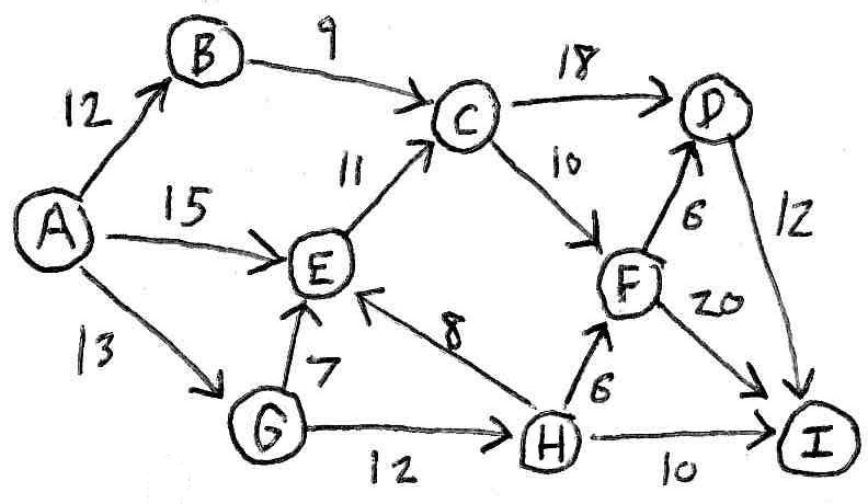
—and dear reader, the maximum-flow problem is solved! For suppose we are faced with the network depicted in the following diagram:

We can then (admittedly with some typing) call for a solution like so:

my_edges = [Edge.new('A', 'B', 12), Edge.new('A', 'E', 15),
  Edge.new('A', 'G', 13), Edge.new('B', 'C', 9), Edge.new('E', 'C', 11),
  Edge.new('G', 'E', 7), Edge.new('C', 'D', 18), Edge.new('C', 'F', 10),
  Edge.new('H', 'E', 8), Edge.new('G', 'H', 12), Edge.new('F', 'D', 6),
  Edge.new('H', 'F', 6), Edge.new('D', 'I', 12), Edge.new('F', 'I', 20),
  Edge.new('H', 'I', 10)]
my_network = FlowNetwork.new('A', 'I', my_edges)
my_network.ford_fulkerson
my_network.report

And receive it like so:

Source: A
Sink: I
A -> B; capacity: 12, flow: 9
A -> E; capacity: 15, flow: 11
A -> G; capacity: 13, flow: 12
B -> C; capacity: 9, flow: 9
E -> C; capacity: 11, flow: 11
G -> E; capacity: 7, flow: 0
C -> D; capacity: 18, flow: 12
C -> F; capacity: 10, flow: 8
H -> E; capacity: 8, flow: 0
G -> H; capacity: 12, flow: 12
F -> D; capacity: 6, flow: 0
H -> F; capacity: 6, flow: 2
D -> I; capacity: 12, flow: 12
F -> I; capacity: 20, flow: 10
H -> I; capacity: 10, flow: 10

Bibliography

Dimitris Bertsimas and John N. Tsitsiklis, Introduction to Linear Optimization, §7.5

Anany Levitin, Introduction to the Design and Analysis of Algorithms, §10.2

Dear reader, I have got to tell you, fandom is intense. One day last October Equestria Daily (internet clearinghouse for fans of the animated series My Little Pony: Friendship Is Magic) posts a joke proposal for a programming language (FIM++) based on the show, and within the week there's a working interpreter for it. What does it mean to model a programming language after a cartoon, you ask? Well, in the show, episodes typically end with our heroine Twilight Sparkle (or after Season Two, Episode Three "Lesson Zero", one of her friends) writing a letter about what she's learned about the magic of friendship to her mentor (and God-Empress of the sun) Princess Celestia. So, then, why not have an esoteric programming langauge where the source code reads like a letter to Princess Celestia? Adorable, right?

So, this gift having been provided to us courtesy of Karol S. and the brony community, let's do something with it! More specifically, how about we implement quicksort?—that is a classic. What's quicksort? Well, we want to sort a list, right? So—bear with me—we define this partitioning procedure that, given indices into an array, partitions the subarray between those indices into a subsubarray of elements less-than-or-equal-to a given element dubbed the pivot, then the pivot itself, then a subsubarray of elements greater than the pivot. How do we do that? Well, let's designate the last element in our subarray as the pivot. Then we're going to scan through all the other elements, and if any of them are less-than-or-equal-to the pivot, we swap it into our first subsubarray and increment a variable keeping track of where the first subsubarray ends. Then, we swap the pivot into place and return its index. In Ruby—

def partition(array, p, r)
  i = p-1
  for j in p..(r-1) do
      if array[j] <= array[r]
        i += 1
        array[i], array[j] = array[j], array[i]
      end
  end
  array[i+1], array[r] = array[r], array[i+1]
  i+1
end

Then we can sort an entire array with a bunch of recursive calls to our partitioning procedure:

def quicksort(array, p, r)
  if p < r
    q = partition(array, p, r)
    quicksort(array, p, q-1)
    quicksort(array, q+1, r)
  end
end

# Let's try it!
my_array = [9, 5, 4, 11, 2, 10, 6, 3, 8, 12, 1, 7]
quicksort(my_array, 0, my_array.length-1)
print my_array # => [1, 2, 3, 4, 5, 6, 7, 8, 9, 10, 11, 12]

So that's quicksort. With a little more effort, we can do the same thing in FIM++:

Dear Princess Celestia: Letter about Quicksort:

I learned about exchange with Applejack, Rainbow Dash, and Rarity.

  On the page numbered by Rarity of Applejack I read about Sweetie
  Belle.

  On the page numbered by Rainbow Dash of Applejack I read about
  Scootaloo.

  On the page numbered by Rarity of Applejack I wrote what I knew
  about Scootaloo.

  On the page numbered by Rainbow Dash of Applejack I wrote what I
  knew about Sweetie Belle.

That's about exchange.


I learned about partitioning with Applejack, Rainbow Dash, and Rarity.

  On the page numbered by Rarity of Applejack I read about Apple
  Bloom.

  Sweetie Belle made the difference of Rainbow Dash and the number one.

  Did you know Scootaloo likes Rainbow Dash?

  I did this while Scootaloo had less than Rarity:

    On the page numbered by Scootaloo of Applejack I read about
    Diamond Tiara.

      When Diamond Tiara had not more than Apple Bloom:

        Sweetie Belle got one more.

        I did exchange of Applejack, Sweetie Belle, and Scootaloo.

      That's what I did.

    Scootaloo got one more.

  That's what I did.

  Sweetie Belle got one more.

  I also caused exchange of Applejack, Sweetie Belle, and Rarity.

That's about partitioning with Sweetie Belle.


I learned about quicksort with Applejack, Rainbow Dash, and Rarity:

  When Rainbow Dash had less than Rarity:

    Fluttershy did partitioning of Applejack, Rainbow Dash, and Rarity.

    Fluttershy got one less.

    I caused quicksort of Applejack, Rainbow Dash, and Fluttershy.

    Fluttershy got two more.

    I caused quicksort of Applejack, Fluttershy, and Rarity.

  That's what I did.

That's about quicksort.


Today I learned:

  Did you know Applejack likes 9, 5, 4, 11, 2, 10, 6, 3, 8, 12, 1, and 7?

  Applejack did dictionary of Applejack.

  I said: Applejack!

  I did quicksort of Applejack, one, and twelve.

  I said: Applejack! 

Your Faithful Student,
Twilight Sparkle

Bibliography Cormen et al., Introduction to Algorithms, third ed'n, §7.1

Dear reader, you know what's way more fun than feeling sad about the nature of the cosmos? Data compression, that's what! Suppose you want to send a message to your friends in a nearby alternate universe, but interuniversal communication bandwidth is very expensive (different universes can't physically interact, so we and our alternate-universe analogues can only communicate by mutually inferring what the other party must be saying, which takes monstrous amounts of computing power and is not cheap), so you need to make your message as brief as possible. Note that 'brief' doesn't just have to do with how long your message is in natural language, it also has to do with how that message is represented over the transuniveral communication channel: indeed, the more efficient the encoding, the more you can afford to say on a fixed budget.

The classic ASCII encoding scheme uses seven bits to represent each character. (Seven?—you ask perplexedly, surely you mean eight? Apparently it was seven in the original version.) Can we do better? Well ... ASCII has a lot of stuff that arguably you don't need that badly. Really, upper and lower case letters? Ampersands, asterisks, backslashes? And don't get me started about those unprintable control characters! If we restrict our message to just the uncased alphabet A through Z plus space and a few punctuation marks, then we can encode our message using only a 32 (= \(2^5\)) character set, at five bits per character.

Can we do better? Seemingly not—\(2^4 = 16\) isn't a big enough character set to cover the alphabet. Unless ...

Unless we abandon the assumption that each character needs to be represented by the same number of bits!

Adopting such a variable-length character encoding scheme couldn't help us if all possible messages were equally likely, but this is manifestly not true of the sort of messages anyone would actually want to send: the letter e is more common than the letter q; the word the more common than the string zkb. We can take advantage of the regularities in the sort of messages people would actually want to send by adopting a variable-length encoding scheme that assigns shorter codes to characters that occur more frequently. But then since we can no longer rely on each n bits (for some fixed n) representing one character, we'll also want our encoding scheme to be prefix-free: no character code should be a prefix of any other. That way, our message is unambiguous: if the message starts with (say) 010, which represents (say) e, then we know that the first character is e, because there won't be any other characters with codes that start with 010 (like say 01011).

Consider the process of decoding a prefix-free code: we read bits from the start of the message until we recognize a valid character code. We can visualize this graphically in the form of a binary tree with the characters in our character set at the leaves: start at the root, and then go the the left child if the first bit is 0, and the right child if it's 1, and so on until you reach a leaf, the path taken representing the code for the character at that leaf. The task of constructing such an optimal such tree (and thereby, an optimal prefix-free code) given the relative frequencies of the characters (either in a particular message, or a general class of messages that people would actually want to send) is solved by a algorithm due to David A. Huffman, which we'll implement here in Python.

First, we'll need a data structure to represent the nodes of the tree. Actually, we'll use a structure that represents a node and all of its children, which we'll call Subtree. Each instance of Subtree will have fields for a character and frequency associated with a node, and the node's left and right children if any (which are also instances of Subtree).

class Subtree:
    def __init__(self, char, freq, left, right):
        self.char = char
        self.freq = freq
        self.left = left
        self.right = right

The leaf nodes of our tree will have the character field set to a character in our set, the frequency field set to the frequency of that character, and the left and right children fields set to None. The internal nodes of the tree will have the character field set to None and the frequency field set to the sum of the frequencies of its children.

We'll also want nodes to be comparable by their frequencies:

    def __gt__(self, othernode):
        return self.freq > othernode.freq

When all is said and done, Huffman's algorithm will give us an instance of Subtree representing our tree, but it would really be more convenient to have the decoding information embodied by the tree in the form of Python dictionary mapping bitstrings to the characters they encode. We can get this by doing a standard recursive tree walk:

    def codebook(self):
        codes = {}
        def traversal(item, code):
            if item != None:
                traversal(item.left, code+'0')
                if item.char != None:
                    codes[item.char] = code
                traversal(item.right, code+'1')
        traversal(self, '')
        return codes

We're also going to need a min-priority queue, a dynamic set from which we can insert items and retrieve the "smallest":

class MinPriorityQueue:
    def __init__(self):
        self.queue = []

    def put(self, item):
        self.queue.append(item)
        self.queue.sort(reverse=True)

    def get(self):
        return self.queue.pop()

Now that we have the appropriate data structures, we're ready for Huffman's algorithm. Suppose our character/frequency data are given to us in a Python dictionary C. For each character, we create an instance of Subtree to be the corresponding leaf node in our tree, and put them all in a min-priority queue. Then we build our tree from the bottom up by selecting the two lowest-frequency nodes in the queue, making them the children of a new node whose frequency is the sum of their frequencies, putting the new node back in the priority queue, and again until we've built the entire tree:

def Huffman(C):
    Q = MinPriorityQueue()
    leaves = {Subtree(k, C[k], None, None) for k in C}
    for leaf in leaves:
        Q.put(leaf)
    for i in range(len(C)-1):
        left = Q.get()
        right = Q.get()
        new_node = Subtree(None, left.freq + right.freq, left, right)
        Q.put(new_node)
    return Q.get().codebook()

And that's Huffman's algorithm. Of course, we'll also want functions for encoding and decoding a message:

def code(plaintext, codebook):
    return ''.join(codebook[c] for c in plaintext)

def decode(ciphertext, codebook):
    decodebook = {v:k for k, v in codebook.items()}
    codeword = ''
    plaintext = ''
    for i in range(len(ciphertext)):
        codeword += ciphertext[i]
        if codeword in decodebook:
            plaintext += decodebook[codeword]
            codeword = ''
    return plaintext

So, suppose you want to send your friends in a nearby alternate universe the eighty-two character message, "I USED TO WONDER WHAT FRIENDSHIP COULD BE, UNTIL YOU ALL SHARED ITS MAGIC WITH ME." If you used seven-bit ASCII, you'd have to pay the cost of transmitting 82*7 = 574 bits. But if you use a Huffman code informed by knowledge of English letter frequencies ...

eng_freqs = {'A' : 8167, 'B' : 1492, 'C' : 2782, 'D' : 4253, 'E' : 12702,
'F' : 2228, 'G' : 2015, 'H' : 6094, 'I' : 6966, 'J' : 153, 'K' : 772,
'L' : 4025, 'M' : 2406, 'N' : 6749, 'O' : 7507, 'P' : 1929, 'Q' : 95,
 'R' : 5987, 'S' : 6327, 'T' : 9056, 'U' : 2758, 'V' : 978, 'W': 2360,
'X' : 150, 'Y' : 1974, 'Z' : 74, ' ' : 13000, '.': 4250, ',': 4250}
eng_codebook = Huffman(eng_freqs)
plain = "I USED TO WONDER WHAT FRIENDSHIP COULD BE, UNTIL YOU ALL SHARED ITS MAGIC WITH ME."
cipher = code(plain, eng_codebook)

You can send this instead:

0111010111100000100111001010110110010101110101001011011001001111110101110100
0001010110101011100111111011100101101100100010000011110000101011110110011111
0010110110010101000000011100001011110001101101011110110010100010100111110001
0101010110101100100001000010101111100111001010011111010001010111011101010001
1011111110101011101001111101000001011101100110111

—which is only 353 bits, for a savings of 38.5%.

Bibliography Cormen et al., Introduction to Algorithms, third ed'n, §16.3