An Algorithmic Lucidity

a blog

Category: mathematics

Discontinuous Linear Functions?!

We know what linear functions are. A function f is linear iff it satisfies additivity f(x + y) = f(x) + f(y) and homogeneity f(ax) = af(x).

We know what continuity is. A function f is continuous iff for all ε there exists a δ such that if |xx0| < δ, then |f(x) − f(x0)| < ε.

An equivalent way to think about continuity is the sequence criterion: f is continuous iff a sequence (xk) converging to x implies that (f(xk)) converges to f(x). That is to say, if for all ε there exists an N such that if kN, then |xkx| < ε, then for all ε, there also exists an M such that if kM, then |f(xk) − f(x)| < ε.

Sometimes people talk about discontinuous linear functions. You might think: that's crazy. I've seen many linear functions in my time, and they were definitely all continuous. f(x): ℝ → ℝ := ax is continuous for any a ∈ ℝ. T(x⃗): ℝ² → ℝ² := \(\begin{pmatrix} a & b \\ c & d \end{pmatrix} \boldsymbol{\vec{v}}\) is continuous no matter what the entries in the matrix are. Stop being crazy!!

Actually, it's not crazy. It's just that all the discontinuous linear functions live in infinite-dimensional spaces.

Take, say, the space C1([a,b]) of continuously differentiable functions from a closed interval [a,b] to ℝ with the uniform norm. (The uniform norm means that the "size" of a function for the purposes of continuity is the least upper bound of its absolute value.) If you think of a vector in the n-dimensional ℝn as a function from {1...n} to ℝ, then you can see why a function from a continuous (not even countable) domain would be infinite-dimensional.

Consider the sequence of functions (fk) = \((\frac{\sin kx}{k})_{k=1}^{\infty}\) in C1([a,b]). The sequence converges to the zero function: for any ε, we can take \(N := \lceil \frac{1}{\varepsilon} \rceil\) and then \(\frac{\sin kx}{k} \le \frac{1}{\lceil \frac{1}{\varepsilon} \rceil} \le \frac{1}{\frac{1}{\varepsilon}} = \varepsilon\).

Now consider that the sequence of derivatives is \((\frac{k \cos kx}{k})_{k=1}^{\infty} = (\cos kx)_{k=1}^{\infty}\), which doesn't converge. But the function D: C1([a,b]) → C0([a,b]) that maps a function to its derivative is linear. (We have additivity because the derivative of a sum is the sum of the derivatives, and we have homogeneity because you can "pull out" a constant factor from the derivative.)

By exhibiting a function D and a sequence (fk) for which (fk) converges but (D(fk)) doesn't, we have shown that the derivative mapping D is a discontinuous linear function, because the sequence criterion for continuity is not satisfied. If you know the definitions and can work with the definitions, it's not crazy to believe in such a thing!

The infinite-dimensionality is key to grasping the ultimate sanity of what would initially have appeared crazy. One way to think about continuity is that a small change in the input can't correspond to an arbitrarily large change in the output.

Consider a linear transformation T on a finite-dimensional vector space; for simplicity of illustration, suppose it's diagonalizable with eigenbasis {u⃗j} and eigenvalues {λj}. Then for input x⃗ = Σj cju⃗j, we have T(x⃗) = Σj cjλju⃗j: the eigencoördinates of the input get multiplied by the eigenvalues, so the amount that the transformation "stretches" the input is bounded by maxjj|. The linearity buys us the "no arbitrarily large change in the output" property which is continuity.

In infinite dimensions, linearity doesn't buy that. Consider the function T(x1, x2, x3, ...) = (x1, 2x2, 3x3, ...) on sequences finitely many nonzero elements, under the uniform norm. The effect of the transformation on any given dimension is linear and bounded, but there's always another dimension that's getting stretched more. A small change in the input can result in an arbitrarily large change in the output, by making the change sufficiently far in the sequence (where the input is getting stretched more and more).

(Thanks to Jeffrey Liang and Gurkenglas for corrections to the original version of this post.)

The End of the Movie: SF State's 2024 Putnam Competition Team, A Retrospective

From: Zack M Davis <zmd@sfsu.edu>
Sent: Sunday, January 12, 2025 11:52 AM
To: math_majors@lists.sfsu.edu <math_majors@lists.sfsu.edu>, math_graduate@lists.sfsu.edu <math_graduate@lists.sfsu.edu>, math_lecturers@lists.sfsu.edu <math_lecturers@lists.sfsu.edu>, math_tenure@lists.sfsu.edu <math_tenure@lists.sfsu.edu>
Subject: the end of the movie: SF State's 2024 Putnam Competition team, a retrospective

Because life is a gradual series of revelations
That occur over a period of time
It's not some carefully crafted story
It's a mess, and we're all gonna die

If you saw a movie that was like real life
You'd be like, "What the hell was that movie about?
It was really all over the place."
Life doesn't make narrative sense

—"The End of the Movie", Crazy Ex-Girlfriend

Every Hollywood underdog story starts with a dream. The scrawny working-class kid who wants to play football for Notre Dame. The charismatic teacher at a majority-Latino school in East L.A. who inspires his class to ace the AP Calculus exam. The debate team at a historically black college that unseats the reigning national champions. Hollywood tells us that if you work hard and believe in yourself, you can defy all expectations and achieve your dream.

Hollywood preys on the philosophically unsophisticated. Chebyshev's inequality states that the probability that a random variable deviates from its mean by more than k standard deviations is no more than 1/k². Well-calibrated expectations already take into account how hard you'll work and how much you'll believe in yourself: underdogs mostly lose by definition.

Accordingly, this story starts with a correspondingly humble dream: the not-a-kid-anymore returning to SFSU after a long absence to finish up his math degree, who wants to get a nonzero score in the famous William Lowell Putnam Mathematical Competition®. (It's not quite as humble as it sounds: the median score in the famously brutal elite competition is often zero out of 120, although last year the median was nine.)

The first step on the road to a nonzero score was being able to compete at all: SF State had no immediate history of participating in the event, in contrast to other schools that devote significant resources to it. (E.g., at Carnegie Mellon, they have a for-credit 3-unit Putnam seminar that meets six days a week.) At SFSU in 2012, I had asked one of my professors about registering for the Putnam, and nothing came of it. This time, a more proactive approach was called for. After reaching out to the chair and several professors who had reasons to decline the role ("I'm not a fan of the Putnam", "I have negative time this semester", "You should ask one of the smart professors"), Prof. Arek Goetz agreed to serve as local supervisor.

A preparation session #1 to discuss the solutions to problems from the 2010 competition was scheduled and aggressively advertised on the math-majors mailing list. (That is, "aggressively" in terms of the rhetoric used, not frequency of posts.) Despite some interest expressed in email, no non-organizer participants showed up, and my flailing attempts at some of the 2010 problems mostly hadn't gotten very far ... but I had at least intuited the correct answer to B2, if not the proof. (We are asked about the smallest possible side of a triangle with integer coordinates; the obvious guess is 3, from the smallest Pythagorean triple 3–4–5; then we "just" have to rule out possible side lengths of 1 and 2.) The dream wasn't dead yet.

To keep the dream alive, recruitment efforts were stepped up. When I happened to overhear a professor in the department lounge rave about a student citing a theorem he didn't know on a "Calculus III" homework assignment, I made sure to get the student's name for a group email to potential competitors. A When2Meet scheduling poll sent to the group was used to determine the time of prep session #2, which was advertised on the department mailing list with a promise of free donuts (which the department generously offered to reïmburse).

Session #2 went well—four participants came, and Prof. Goetz made an appearance. I don't think we made much progress understanding the 2011 solutions in the hour before we had to yield TH 935 to the Ph.D. application group, but that wasn't important. We had four people. This was really happening!

As the semester wore on, the group kept in touch on our training progress by email, and ended up holding three more in-person sessions as schedules permitted (mean number of attendees: 1.67). Gelca and Andreescu's Putnam and Beyond was a bountiful source of practice problems in addition to previous competitions.

Finally, it was Saturday 7 December. Gameday—exam day, whatever. Three competitors (including one who hadn't been to any of the previous prep sessions), gathered in the Blakeslee room at the very top of Thornton Hall to meet our destiny. The Putnam is administered in two sessions: three hours in the morning (problems identified as A1 through A6 in roughly increasing difficulty), and three hours in the afternoon (problems B1 through B6).

Destiny was not kind in the problem selection for the "A" session.

A1 was number theory, which I don't know (and did not, unfortunately, learn from scratch this semester just for the Putnam).

I briefly had some hope for B2, which asked for which real polynomials p is there a real polynomial q such that p(p(x)) − x = (p(x) − x)²q(x). If I expanded the equation to Σj=0n ajk=0n ak xk)j − x = (Σj=0n aj xj − x)² Σj=1n bj xj, and applied the multinomial theorem ... it produced a lot of impressive Σ–Π index notation, but didn't obviously go anywhere towards solving the problem.

A3 was combinatorics. Concerning the set S of bijections T from {1, 2, 3} × {1, 2, ..., 2024} to {1, 2, ..., 6072} such that T(1, j) < T(2, j) < T(3, j) and T(i, j) < T(i, j+1), was there an a and c in {1, 2, 3} and b and d in {1, 2, ..., 2024} such that the fraction of elements T in S for which T(a, b) < T(c, d) is at least ⅓ and at most ⅔? I couldn't get a good grasp on the structure of S (e.g., how many elements it has), which was a blocker to being able to say something what fraction of it fulfills some property. Clearly a lexicographic sort by the first element, or by the second element, would fulfill the inequalities, but how many other bijections were in S? When the solutions were later published, the answer turned out to involve a standard formula about Young tableaus, not something I could have realistically derived from scratch during the exam.

A4 was more number theory; I didn't even read it. (I still haven't read it.)

A5 asked about how to place a radius-1 disc inside a circle of radius 9 in order to minimize the probability that a chord through two uniformly random points on the circle would pass through the disk. I recognized the similarity to Bertrand's paradox and intuited that a solution would probably be at one of the extremes, putting the disc at the center or the edge. There was obviously no hope of me proving this during the exam. (It turned out to be the center.)

A6 was a six; I didn't read it.

I turned in pages with my thoughts on A2, A3, and A5 because it felt more dignified than handing in nothing, but those pages were clearly worth zero points. The dream was dying.

Apparently I wasn't the only one demoralized by the "A" problems; the other competitors didn't return for the afternoon session. Also, it turned out that we had locked ourselves out of the Blakeslee room, so the afternoon session commenced with just me in TH 935, quietly hoping for a luckier selection of "B" problems, that this whole quixotic endeavor wouldn't all have been for nothing.

Luck seemed to deliver. On a skim, B1, B2, and B4 looked potentially tractable. B2 was geometry, and I saw an angle of attack (no pun intended) ...

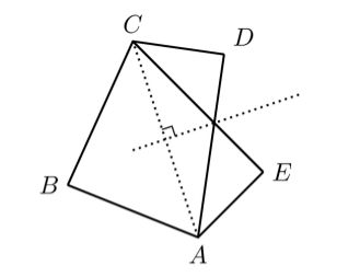
B2. Two convex quadrilaterals are called partners if they have three vertices in common and they can be labeled ABCD and ABCE so that E is the reflection of D across the perpendicular bisector of the diagonal AC. Is there an infinite sequence of convex quadrilaterals such that each quadrilateral is a partner of its successor and no two elements of the sequence are congruent?

diagram of two partner quadrilaterals sharing vertices A, B, C, labeled ABCD and ABCE, with D and E reflected across the perpendicular bisector of diagonal AC

I imagined rotating the figure such that AC was the vertical axis and its bisector was the horizontal axis, and tried to imagine some way to perturb D and E to get a sequence of quadrilaterals that wouldn't be congruent (because the angles ∠CDA and ∠CEA were changing), but for which we could alternately take ABCD and ABCE so that successive shapes in the sequence would be partners. I couldn't see a way to make it work. Then I thought, what if perturb B instead?

Yes, I began to write excitedly, there exists such a sequence. For example, in ℝ², let A := (0, −1), C := (0, 1), D := (½, ½), and E := (½, −½), and consider a sequence Bn on the unit circle strictly in quadrant II (i.e., with x < 0 and y > 0), for example, Bn := (Re exp((π - 1/n)i), Im exp((π - 1/n)i)) where ℝ² is identified with ℂ. Then consider the sequence of quadrilaterals ABnCD for odd n and ABnCE for even n, for n ∈ ℕ+. Successive quadrilaterals in the sequence are partners: the perpendicular bisector of the diagonal AC is the x-axis, and D = (½, ½) and E = (½, −½) are reflections of each other across the x-axis. No two quadrilaterals in the sequence are congruent because the angle ∠ABnC is different for each n ...

Or is it? I recalled a fact from Paul Lockhart's famous lament: somewhat counterintuitively, any triangle inscribed in a 0ylsemicircle is a right triangle: ∠ABnC would be the same for all n. (The quadrilaterals would still be different, but I would have to cite some other difference to prove it.) I took a fresh piece of paper and rewrote the proof with a different choice of Bn: instead of picking a sequence of points on the unit circle, I chose a sequence on the line y = x + 1: say, Bn := (−1/(n+1), 1 − 1/(n+1)). Then I could calculate the distance AB as √(1/(n+1)² + (1 − 1/(n+1))²), observe that the angle ∠BCA was 45°, invoke the law of sines to infer that the ratio of the sine of ∠ABC to the distance AC (viz., 2) was equal to the ratio of the sine of ∠BCA (viz., √2/2) to the distance AB, and infer that ∠ABC is arcsin(√2/AB‾), and therefore that the quadrilaterals in my sequence were not congruent. Quod erat demonstrandum!

That took the majority of my time for the afternoon session; I spent the rest of it tinkering with small-n cases for B1 and failing to really get anywhere. But that didn't matter. I had solved B2, hadn't I? That had to be a solve, right?—maybe 8 points for less than immaculate rigor, but not zero or one.

Last year the published contest results only listed the names of top 250 individuals, top 10 teams, and top 3 teams by MAA section ("Golden Section: Stanford University; University of California, Berkeley; University of California, Davis"), but I fantasized about looking up who I should write to at the MAA to beg them to just publish the full team scores. Who was privacy helping? People who go to R2 universities already know that we're stupid. Wouldn't it be kinder to at least let us appear at the bottom of the list, rather than pretending we didn't exist at all? All weekend, in the movie of my life in my head, I could hear the sports announcer character (perhaps portrayed by J. K. Simmons) crowing: Gators on the board! Gators on the board!

All weekend and until the embargo period ended on 10 December and people began discussing the answers online, reminding me that real life isn't a movie.

I did not write to the MAA.

The Gators were not on the board.

I did not solve B2.

The answer is No, there is no such sequence of quadrilaterals. The Putnam archive solutions and a thread on the Art of Problem Solving forums explain how to prove it.

As for my "proof", well, the problem statement said that partner quadrilaterals have three vertices in common. In my sequence, successive elements ABnCD and ABn+1CE have two vertices in common, A and C.

This isn't a fixable flaw. If you have the reading comprehension to understand the problem statement, the whole approach just never made any sense to begin with. If it made sense to me while I was writing it, well—what's that phrase mathematicians like to use? Modus tollens.

You could say that there's always next year—but there isn't, for me. Only students without an undergraduate degree are eligible to take the Putnam, and I'm graduating next semester. (In theory, I could delay it and come back in Fall 2025, but I'm already graduating fifteen years late, and no humble dream is worth making it fifteen and a half.)

I keep wanting to believe that this isn't the end of the movie. Maybe this year's effort was just the first scene. Maybe someone reading this mailing list post will hear the call to excellence and assemble a team next year that will score a point—not out of slavish devotion to Putnam competition itself, but to what it represents, that there is a skill of talking precisely about precise things that's worth mastering—that can be mastered by someone trying to master it, which mastery can be measured by a wide-ranging test with a high ceiling and not just dutiful completion of course requirements.

Maybe then this won't all have been for nothing.

Recruitment Advertisements for the 2024 Putnam Competition at San Francisco State University

From: Zack M Davis <zmd@sfsu.edu>
Sent: Wednesday, September 11, 2024 5:02 PM
To: math_majors@lists.sfsu.edu <math_majors@lists.sfsu.edu>
Subject: Putnam prep session for eternal mathematical glory, 4 p.m. Thu 19 September

One must make a distinction however: when dragged into prominence by half-poets, the result is not poetry, nor till the poets among us can be "literalists of the imagination"—above insolence and triviality and can present for inspection "imaginary gardens with real toads in them", shall we have it. In the meantime, if you demand on the one hand the raw material of poetry in all its rawness, and that which is on the other hand genuine, then you are interested in poetry.

—Marianne Moore

The William Lowell Putnam Mathematical Competition, the renowned annual math examination for undergraduates with cash prizes for top performers, is to be held on Saturday, 7 December 2024. Registration details will be available soon, but for now, potential competitors are invited to come to an initial preparatory/training session at 4 p.m. on Thursday, September 19th in the math department conference room TH 935.

To get the most out of it, try struggling with some of the problems from the 2010 competition beforehand: we'll discuss solutions and strategies together at the meeting. (The problems are numbered A1–A6 and B1–B6, corresponding to the morning and afternoon sessions of the competition; the earlier-numbered problems within each are supposed to be easier.) If you can't make this time but are interested in the endeavor, I want to hear from you: email me at zmd@sfsu.edu.

"FREQUENTLY" ASKED QUESTIONS

Q: Did you say "cash prizes"? I'm pretty good at math: I got an "A" in MATH 228. Should I participate in hopes of winning?

A: No. No one who goes to SF State is going to win any prizes. The Putnam is an elite competition designed to test the abilities of the finest young mathematical minds in the world. The graders are notoriously stingy about awarding partial credit: the median score is often zero points out of 120. Last year seems to have been a bit easier: the median score was 9.1 Of the top sixteen scorers, thirteen went to MIT.

Q: Wait, this sounds awful. I'm already spending way too much of my life shuffling formulæ around just to keep up with my classes. You're asking me to spend even more of my precious time attempting insanely difficult problems, to prepare for a six-hour exam three months from now that I have no hope of doing well on, and it wouldn't even earn credit for my degree? Why would I do that?

A: Because it doesn't earn credit for your degree. The Putnam isn't an obedience test where a designated bureaucratic authority figure commands you to use a fixed set of methods to solve a fixed set of problems in exchange for a piece of paper with an "A" written on it. It's a challenge of your creativity, breadth of knowledge, and determination—a Schelling point for those who demand the raw material of mathematics and that which is on the other hand genuine to prove to ourselves and the world what we're capable of. If you're afraid of what you'll learn about yourself by trying, then don't.

1: The Duke Research Blog reports that there were 3,857 competitors in 2023, and the official results report that 2,200 contests scored higher than 9 and 1,610 scored higher than 10.


From: Zack M Davis <zmd@sfsu.edu>
Sent: Sunday, September 29, 2024 11:17 PM
To: math_majors@lists.sfsu.edu <math_majors@lists.sfsu.edu>
Subject: Putnam prep session #2 for eternal mathematical glory ... and donuts, 2 p.m. Fri 4 October

"Hey, Goofusia," said Gallantina. "Did you see this post on the math_majors list? Someone's trying to organize a team for the Putnam competition—here, at SFSU! There's going to be a prep session in Thornton 935 on Friday at 2 p.m. The organizer sounds really desperate—there should be free donuts. Want to come?"

Fraternal twins, the sisters looked so much alike that strangers who didn't know them often asked if they were identical. People who knew them for any length of time never asked.

Goofusia grimaced. "Oh, God, is that that super-hard math competition that guys from MIT win every year, where the median score is zero?"

"Actually, someone not from MIT won as recently as 2018, and last year the median score was nine. But yes."

"Uh-huh. What school was the 2018 winner from?"

"Um, Harvard."

"I'll pass. You should, too."

"C'mon, it'll be fun!"

"Gallantina, you don't know what fun is. You're so caught up in your delusional self-image of pro-sociality that you can't even notice what you actually enjoy." Goofusia spoke with a firm emphasis and cadence, "I, am learning math, in order to get grades, in order to get a degree, in order to get a job. So is everyone else in our major. So are you. That's the only possible reason—the only human reason. You just can't admit it to yourself—"

"That's not true!"

"—and you're so fanatically devoted to maintaining your false self-image as some intrinsically motivated student of the cosmos that you're willing to torture yourself with more schoolwork that doesn't even benefit you. You are not going to score points on the Putnam—"

"I might!" said Gallantina steadfastly, suddenly turning away from three walls of the room to face the remaining one and looking past Goofusia as if to speak to someone else. "With dedication and practice, and with the help of all the lifelong friends I'll make in TH 935 at 2 p.m. this Friday October fourth!"

"Spare me. What does prepping for an impossible exam even look like?"

"Well, the idea is that before the meeting, I and others will prepare at home by trying problems from the 2011 competition with however much time we choose to spare for the task, and then at the meeting, we'll compare answers and discuss the published solutions."

"If any of you losers even come up with any answers to compare."

"We might! I've already made some partial progress on the first problem."

"You don't have to tell m—" Goofusia tried to say, but Gallantina had already begun to read:

A1. Define a growing spiral in the plane to be a sequence of points with integer coordinates P0 = (0, 0), P1, ..., Pn such that n ≥ 2 and:
• the directed line segments P0–P1, P1–P2, ..., P(n−1)–Pn are in the successive coordinate directions east (for P0–P1), north, west, south, east, etc.;
• the lengths of these line segments are positive and strictly increasing.

How many of the points (x, y) with integer coordinates 0 ≤ x ≤ 2011, 0 ≤ y ≤ 2011 cannot be the last point, Pn of any growing spiral?

"Two thousand and eleven?" Goofusia asked disdainfully.

"They like to work the competition year into one of the problem statements. I think it's cute," said Gallantina. "Anyway, I started thinking about the minimal growing spiral—one step east, two steps north, three steps west, &c. The x-coördinate steps are 1, -3, 5, -7 ..., the y-coördinate steps are 2, -4, 6, -8 ..., the x-coördinate net endpoints are 1, -2, 3, -4, 5 ... and the y-coördinate net endpoints are 2, -2, 4, -4, ... There are more possible spirals besides the minimal one, of course, but we can already see there are patterns in what endpoints are possible."

"You're wasting your time," said Goofusia. "Precisely because the question asks about all possible growing spirals, you're not going to learn anything by examining particular cases. You can immediately see that any point with an x-coördinate less than the y-coördinate will do: just take x steps east and y steps north."

Gallantina was beaming.

"Wh—what are you smiling at?"

Gallantina nodded, still beaming.

Goofusia scowled. "Whatever," she said, and turned to leave, then stopped. "So ... what's the answer?"

Gallantina shrugged. "We haven't finished solving it yet. But if it turns out to be beyond us, I'm sure they'll tell us in TH 935 at 2 p.m. this Friday October fourth."

Goofusia shook her head. "I couldn't possibly. I have an exam this week, and a lot of homework."

"But you don't specifically have anything else going on at 2 on Friday? They're notoriously hard problems, and everyone is busy. There'd be no shame in showing up and eating a donut without having successfully solved anything at home."

"No, I mean that's not who I am. I'm not like you. I'm a student at SF State, not—not the cosmos!"

Goofusia left. Alone, Gallantina addressed the fourth wall again. "Is that who you are?"

Bayesian Networks Aren’t Necessarily Causal

(originally published at Less Wrong)

As a casual formal epistemology fan, you've probably heard that the philosophical notion of causality can be formalized in terms of Bayesian networks—but also as a casual formal epistemology fan, you also probably don't know the details all that well.

One day, while going through the family archives, you come across a meticulously maintained dataset describing a joint probability distribution over four variables: whether it rained that day, whether the sprinkler was on, whether the sidewalk was wet, and whether the sidewalk was slippery. The distribution is specified in this table (using the abbreviated labels "rain", "slippery", "sprinkler", and "wet"):

$$\begin{matrix} \mathrm{rain}=\mathrm{True},\, \mathrm{slippery}=\mathrm{True},\, \mathrm{sprinkler}=\mathrm{True},\, \mathrm{wet}=\mathrm{False} & \frac{1}{140000} \approx 0.0000 \cr \mathrm{rain}=\mathrm{False},\, \mathrm{slippery}=\mathrm{True},\, \mathrm{sprinkler}=\mathrm{True},\, \mathrm{wet}=\mathrm{False} & \frac{3}{14000} \approx 0.0002 \cr \mathrm{rain}=\mathrm{True},\, \mathrm{slippery}=\mathrm{True},\, \mathrm{sprinkler}=\mathrm{False},\, \mathrm{wet}=\mathrm{False} & \frac{3}{14000} \approx 0.0002 \cr \mathrm{rain}=\mathrm{True},\, \mathrm{slippery}=\mathrm{False},\, \mathrm{sprinkler}=\mathrm{True},\, \mathrm{wet}=\mathrm{False} & \frac{99}{140000} \approx 0.0007 \cr \mathrm{rain}=\mathrm{False},\, \mathrm{slippery}=\mathrm{False},\, \mathrm{sprinkler}=\mathrm{False},\, \mathrm{wet}=\mathrm{True} & \frac{9}{5600} \approx 0.0016 \cr \mathrm{rain}=\mathrm{False},\, \mathrm{slippery}=\mathrm{True},\, \mathrm{sprinkler}=\mathrm{False},\, \mathrm{wet}=\mathrm{True} & \frac{27}{5600} \approx 0.0048 \cr \mathrm{rain}=\mathrm{False},\, \mathrm{slippery}=\mathrm{True},\, \mathrm{sprinkler}=\mathrm{False},\, \mathrm{wet}=\mathrm{False} & \frac{891}{140000} \approx 0.0064 \cr \mathrm{rain}=\mathrm{True},\, \mathrm{slippery}=\mathrm{False},\, \mathrm{sprinkler}=\mathrm{True},\, \mathrm{wet}=\mathrm{True} & \frac{7}{800} \approx 0.0088 \cr \mathrm{rain}=\mathrm{False},\, \mathrm{slippery}=\mathrm{False},\, \mathrm{sprinkler}=\mathrm{True},\, \mathrm{wet}=\mathrm{False} & \frac{297}{14000} \approx 0.0212 \cr \mathrm{rain}=\mathrm{True},\, \mathrm{slippery}=\mathrm{False},\, \mathrm{sprinkler}=\mathrm{False},\, \mathrm{wet}=\mathrm{False} & \frac{297}{14000} \approx 0.0212 \cr \mathrm{rain}=\mathrm{False},\, \mathrm{slippery}=\mathrm{False},\, \mathrm{sprinkler}=\mathrm{True},\, \mathrm{wet}=\mathrm{True} & \frac{3}{140} \approx 0.0214 \cr \mathrm{rain}=\mathrm{True},\, \mathrm{slippery}=\mathrm{True},\, \mathrm{sprinkler}=\mathrm{True},\, \mathrm{wet}=\mathrm{True} & \frac{21}{800} \approx 0.0262 \cr \mathrm{rain}=\mathrm{True},\, \mathrm{slippery}=\mathrm{False},\, \mathrm{sprinkler}=\mathrm{False},\, \mathrm{wet}=\mathrm{True} & \frac{27}{560} \approx 0.0482 \cr \mathrm{rain}=\mathrm{False},\, \mathrm{slippery}=\mathrm{True},\, \mathrm{sprinkler}=\mathrm{True},\, \mathrm{wet}=\mathrm{True} & \frac{9}{140} \approx 0.0643 \cr \mathrm{rain}=\mathrm{True},\, \mathrm{slippery}=\mathrm{True},\, \mathrm{sprinkler}=\mathrm{False},\, \mathrm{wet}=\mathrm{True} & \frac{81}{560} \approx 0.1446 \cr \mathrm{rain}=\mathrm{False},\, \mathrm{slippery}=\mathrm{False},\, \mathrm{sprinkler}=\mathrm{False},\, \mathrm{wet}=\mathrm{False} & \frac{88209}{140000} \approx 0.6301 \cr \end{matrix}$$

(You wonder what happened that one day out of 140,000 when it rained, and the sprinkler was on, and the sidewalk was slippery but not wet. Did—did someone put a tarp up to keep the sidewalk dry, but also spill slippery oil, which didn't count as being relevantly "wet"? Also, 140,000 days is more than 383 years—were "sprinklers" even a thing in the year 1640 C.E.? You quickly put these questions out of your mind: it is not your place to question the correctness of the family archives.)

You're slightly uncomfortable with this unwieldy sixteen-row table. You think that there must be some other way to represent the same information, while making it clearer that it's not a coincidence that rain and wet sidewalks tend to co-occur.

You've read that Bayesian networks "factorize" an unwieldly joint probability distribution into a number of more compact conditional probability distributions, related by a directed acyclic graph, where the arrows point from "cause" to "effect". (Even a casual formal epistemology fan knows that much.) The graph represents knowledge that each variable is conditionally independent of its non-descendants given its parents, which enables "local" computations: given the values of just a variable's parents in the graph, we can compute a conditional distribution for that variable, without needing to consider what is known about other variables elsewhere in the graph ...

You've read that, but you've never actually done it before! You decide that constructing a Bayesian network to represent this distribution will be a useful exercise.

To start, you re-label the variables for brevity. (On a whim, you assign indices in reverse-alphabetical order: \(X_1\) = wet, \(X_2\) = sprinkler, \(X_3\) = slippery, \(X_4\) = rain.)

$$\begin{matrix} X_1=\mathrm{False},\: X_2=\mathrm{True},\: X_3=\mathrm{True},\: X_4=\mathrm{True} & \frac{1}{140000} \cr X_1=\mathrm{False},\: X_2=\mathrm{True},\: X_3=\mathrm{True},\: X_4=\mathrm{False} & \frac{3}{14000} \cr X_1=\mathrm{False},\: X_2=\mathrm{False},\: X_3=\mathrm{True},\: X_4=\mathrm{True} & \frac{3}{14000} \cr X_1=\mathrm{False},\: X_2=\mathrm{True},\: X_3=\mathrm{False},\: X_4=\mathrm{True} & \frac{99}{140000} \cr X_1=\mathrm{True},\: X_2=\mathrm{False},\: X_3=\mathrm{False},\: X_4=\mathrm{False} & \frac{9}{5600} \cr X_1=\mathrm{True},\: X_2=\mathrm{False},\: X_3=\mathrm{True},\: X_4=\mathrm{False} & \frac{27}{5600} \cr X_1=\mathrm{False},\: X_2=\mathrm{False},\: X_3=\mathrm{True},\: X_4=\mathrm{False} & \frac{891}{140000} \cr X_1=\mathrm{True},\: X_2=\mathrm{True},\: X_3=\mathrm{False},\: X_4=\mathrm{True} & \frac{7}{800} \cr X_1=\mathrm{False},\: X_2=\mathrm{True},\: X_3=\mathrm{False},\: X_4=\mathrm{False} & \frac{297}{14000} \cr X_1=\mathrm{False},\: X_2=\mathrm{False},\: X_3=\mathrm{False},\: X_4=\mathrm{True} & \frac{297}{14000} \cr X_1=\mathrm{True},\: X_2=\mathrm{True},\: X_3=\mathrm{False},\: X_4=\mathrm{False} & \frac{3}{140} \cr X_1=\mathrm{True},\: X_2=\mathrm{True},\: X_3=\mathrm{True},\: X_4=\mathrm{True} & \frac{21}{800} \cr X_1=\mathrm{True},\: X_2=\mathrm{False},\: X_3=\mathrm{False},\: X_4=\mathrm{True} & \frac{27}{560} \cr X_1=\mathrm{True},\: X_2=\mathrm{True},\: X_3=\mathrm{True},\: X_4=\mathrm{False} & \frac{9}{140} \cr X_1=\mathrm{True},\: X_2=\mathrm{False},\: X_3=\mathrm{True},\: X_4=\mathrm{True} & \frac{81}{560} \cr X_1=\mathrm{False},\: X_2=\mathrm{False},\: X_3=\mathrm{False},\: X_4=\mathrm{False} & \frac{88209}{140000} \cr \end{matrix}$$

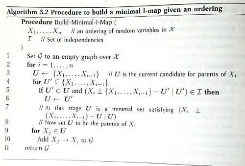
Now, how do you go about building a Bayesian network? As a casual formal epistemology fan, you are proud to own a copy of the book by Daphne Koller and the other guy, which explains how to do this in—you leaf through the pages—probably §3.4, "From Distributions to Graphs"?—looks like ... here, in Algorithm 3.2. It says to start with an empty graph, and it talks about random variables, and setting directed edges in the graph, and you know from chapter 2 that the ⟂ and | characters are used to indicate conditional independence. That has to be it.
textbook page showing "Algorithm 3.2: Procedure to build a minimal I-map given an ordering" pseudocode

(As a casual formal epistemology fan, you haven't actually read chapter 3 up through §3.4, but you don't see why that would be necessary, since this Algorithm 3.2 pseudocode is telling you what you need to do.)

It looks like the algorithm says to pick a variable, allocate a graph node to represent it, find the smallest subset of the previously-allocated variables such that the variable represented by the new node is conditionally independent of the other previously-allocated variables given that subset, and then draw directed edges from each of the nodes in the subset to the new node?—and keep doing that for each variable—and then compute conditional probability tables for each variable given its parents in the resulting graph?

That seems complicated when you say it abstractly, but you have faith that it will make more sense as you carry out the computations.

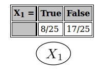
First, you allocate a graph node for \(X_1\). It doesn't have any parents, so the associated conditional ("conditional") probability distribution, is really just the marginal distribution for \(X_1\).
node X₁ with its marginal probability table: P(X₁=True)=8/25, P(X₁=False)=17/25

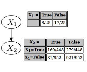
Then you allocate a node for \(X_2\). \(X_2\) is not independent of \(X_1\). (Because \(P(X_1 \land X_2)\) = 169/1400, which isn't the same as \(P(X_1) \cdot P(X_2)\) = 8/25 · 1/7 = 8/175.) So you make \(X_1\) a parent of \(X_2\), and your conditional probability table for \(X_2\) separately specifies the probabilities of \(X_2\) being true or false, depending on whether \(X_1\) is true or false.
graph with an arrow from node X₁ to node X₂, alongside X₁'s marginal table and X₂'s conditional probability table given X₁

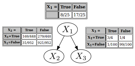
Next is \(X_3\). Now that you have two possible parents, you need to check whether conditioning on either of \(X_1\) and \(X_2\) would render \(X_3\) conditionally independent of the other. If not, then both \(X_1\) and \(X_2\) will be parents of \(X_3\); if so, then the variable you conditioned on will be the sole parent. (You assume that the case where \(X_3\) is just independent from both \(X_1\) and \(X_2\) does not pertain; if that were true, \(X_3\) wouldn't be connected to the rest of the graph at all.)

It turns out that \(X_3\) and \(X_2\) are conditionally independent given \(X_1\). That is, \(P(X_3 \land X_2 \mid X_1) = P(X_3 \mid X_1) \cdot P(X_2 \mid X_1)\). (Because the left-hand side is \(\frac{P(X_3 \land X_2 \land X_1)}{P(X_1)} = \frac{507}{1792}\), and the right-hand side is \(\frac{3}{4} \cdot \frac{169}{448} = \frac{507}{1792}\).) So \(X_1\) is a parent of \(X_3\), and \(X_2\) isn't; you draw an arrow from \(X_1\) (and only \(X_1\)) to \(X_3\), and compile the corresponding conditional probability table.
graph with X₁ as parent of both X₂ and X₃, alongside conditional probability tables for X₂ and X₃ given X₁

Finally, you have \(X_4\). The chore of finding the parents is starting to feel more intuitive now. Out of the \(2^3 = 8\) possible subsets of the preceding variables, you need to find the smallest subset, such that conditioning on that subset renders \(X_4\) (conditionally) independent of the variables not in that subset. After some calculations that the authors of expository blog posts have sometimes been known to callously leave as an exercise to the reader, you determine that \(X_1\) and \(X_2\) are the parents of \(X_4\).

And with one more conditional probability table, your Bayesian network is complete!
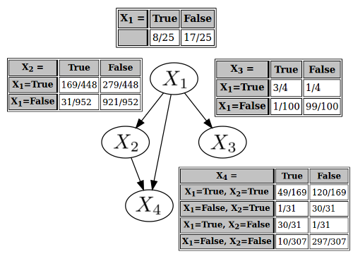
completed four-node graph: X₁ points to X₂ and X₃, and X₁ together with X₂ point to X₄, alongside all four conditional probability tables

Eager to interpret the meaning of this structure regarding the philosophy of causality, you translate the \(X_i\) variable labels back to English:
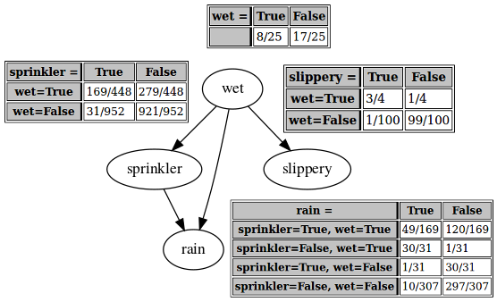
same four-node graph with variables relabeled by their English names: "wet" points to "sprinkler" and "slippery", and "wet" together with "sprinkler" point to "rain"

...

This can't be right. The arrow from "wet" to "slippery" seems fine. But all the others are clearly absurd. Wet sidewalks cause rain? Sprinklers cause rain? Wet sidewalks cause the sprinkler to be on?

You despair. You thought you had understood the algorithm. You can't find any errors in your calculations—but surely there must be some? What did you do wrong?

After some thought, it becomes clear that it wasn't just a calculation error: the procedure you were trying to carry out couldn't have given you the result you expected, because it never draws arrows from later-considered to earlier-considered variables. You considered "wet" first. You considered "rain" last, and then did independence tests to decide whether or not to draw arrows from "wet" (or "sprinkler" or "slippery") to "rain". An arrow from "rain" to "wet" was never a possibility. The output of the algorithm is sensitive to the ordering of the variables.

(In retrospect, that probably explains the "given an ordering" part of Algorithm 3.2's title, "Procedure to build a minimal I-map given an ordering." You hadn't read up through the part of chapter 3 that presumably explains what an "I-map" is, and had disregarded the title as probably unimportant.)

You try carrying out the algorithm with the ordering "rain", "sprinkler", "wet", "slippery" (or \(X_4\), \(X_2\), \(X_1\), \(X_3\) using your \(X_i\) labels from before), and get this network:
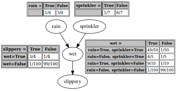
alternate Bayesian network built using the ordering rain, sprinkler, wet, slippery: "rain" and "sprinkler" both point to "wet", which points to "slippery"

—for which giving the arrows a causal interpretation seems much more reasonable.

You notice that you are very confused. The "crazy" network you originally derived, and this "true" network derived from a more intuitively causal variable ordering, are different: they don't have the same structure, and (except for the wet → slippery link) they don't have the same conditional probability tables. You would assume that they can't "both be right". If the network output by the algorithm depends on what variable ordering you use, how are you supposed to know which ordering is correct? In this example, you know from reasons outside the math, that "wet" shouldn't cause "rain", but you couldn't count on that were you to apply these methods to problems further removed from intuition.

Playing with both networks, you discover that despite their different appearances, they both seem to give the same results when you use them to calculate marginal or conditional probabilities. For example, in the "true" network, \(P(\mathrm{rain})\) is 1/4 (read directly from the "conditional" probability table, as "rain" has no parents in the graph). In the "crazy" network, the probability of rain can be computed as

$$P(\mathrm{rain} \mid \mathrm{sprinkler}, \mathrm{wet}) \cdot P(\mathrm{sprinkler} \mid \mathrm{wet}) \cdot P(\mathrm{wet}) +$$
$$P(\mathrm{rain} \mid \neg \mathrm{sprinkler}, \mathrm{wet}) \cdot P(\neg \mathrm{sprinkler} \mid \mathrm{wet}) \cdot P(\mathrm{wet}) +$$
$$P(\mathrm{rain} \mid \mathrm{sprinkler}, \neg \mathrm{wet}) \cdot P(\mathrm{sprinkler} \mid \neg \mathrm{wet}) \cdot P(\neg \mathrm{wet}) +$$
$$P(\mathrm{rain} \mid \neg \mathrm{sprinkler}, \neg \mathrm{wet}) \cdot P(\neg \mathrm{sprinkler} \mid \neg \mathrm{wet}) \cdot P(\neg \mathrm{wet})$$
$$= \frac{49}{169} \cdot \frac{169}{448} \cdot \frac{8}{25} + \frac{30}{31} \cdot \frac{279}{448} \cdot \frac{8}{25} + \frac{1}{31} \cdot \frac{31}{952} \cdot \frac{17}{25} + \frac{10}{307} \cdot \frac{921}{952} \cdot \frac{17}{25}$$

... which also equals 1/4.

That actually makes sense. You were wrong to suppose that the two networks couldn't "both be right". They are both right; they both represent the same joint distribution. The result of the algorithm for constructing a Bayesian network—or a "minimal I-map", whatever that is—depends on the given variable ordering, but since the algorithm is valid, each of the different possible results is also valid.

But if the "crazy" network and the "true" network are both right, what happened to the promise of understanding causality using Bayesian networks?! (You may only be a casual formal epistemology fan, but you remember reading a variety of secondary sources unanimously agreeing that this was a thing; you're definitely not misremembering or making it up.) If both networks give the same answers to marginal and conditional probability queries, that amounts to them making the same predictions about the world. So if beliefs are supposed to correspond to predictions, in what sense could the "true" network be better? What does your conviction that rain causes wetness even mean, if someone who believed the opposite could make all the same predictions?

You remember the secondary sources talking about interventions on causal graphs: severing a node from its parents and forcing it to take a particular value. And the "crazy" network and the "true" network do differ with respect to that operation: in the "true" network, setting "wet" to be false—you again imagine putting a tarp up over the sidewalk—wouldn't change the probability of "rain". But in the "crazy" network, forcing "wet" to be false would change the probability of rain—to \(P(\mathrm{rain} \mid \mathrm{sprinkler}, \neg \mathrm{wet}) \cdot P(\mathrm{sprinkler} \mid \neg \mathrm{wet}) + P(\mathrm{rain} \mid \neg \mathrm{sprinkler}, \neg \mathrm{wet}) \cdot P(\neg \mathrm{sprinkler} \mid \neg \mathrm{wet})\), which is \(\frac{1}{31} \cdot \frac{31}{952} + \frac{10}{307} \cdot \frac{921}{952} \approx 0.032\) (greatly reduced from the 1/4 you calculated a moment ago). Notably, this intervention—\(P(\mathrm{rain} \mid \mathrm{do}(\neg \mathrm{wet}))\), if you're remembering correctly what some of the secondary sources said about a do operator—isn't the same thing as the conditional probability \(P(\mathrm{rain}| \neg \mathrm{wet})\).

This would seem to satisfy your need for a sense in which the "true" network is "better" than the "crazy" network, even if Algorithm 3.2 indifferently produces either depending on the ordering it was given. (You're sure that Daphne Koller and the other guy have more to say about other algorithms that can make finer distinctions, but this feels like enough studying for one day—and enough for one expository blog post, if someone was writing one about your inquiries. You're a casual formal epistemology fan.) The two networks represent the same predictions about the world recorded in your family archives, but starkly different predictions about nearby possible worlds—about what would happen if some of the factors underlying the world were to change.

You feel a slight philosophical discomfort about this. You don't like the idea of forced change, of intervention, being so integral to such a seemingly basic notion as causality. It feels almost anthropomorphic: you want the notion of cause and effect within a system to make sense without reference to the intervention of some outside agent—for there's nothing outside of the universe. But whether this intuition is a clue towards deeper insights, or just a place where your brain has tripped on itself and gotten confused, it's more than you understand now.
The Univariate Fallacy

(originally published at Less Wrong)

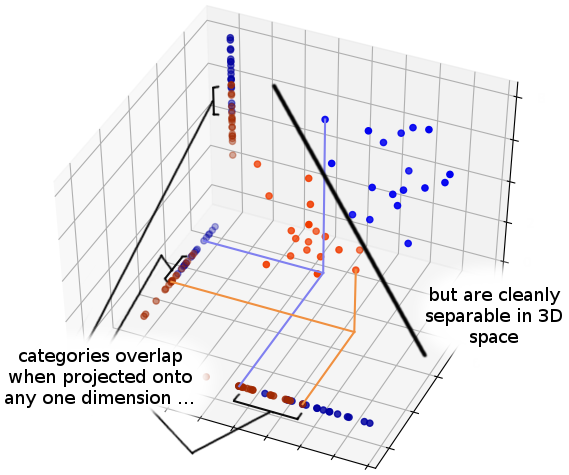
There's this statistical phenomenon where it's possible for two multivariate distributions to overlap along any one variable, but be cleanly separable when you look at the entire configuration space at once. This is perhaps easiest to see with an illustrative diagram—

3D scatterplot of two colored point clusters that overlap when projected onto any single axis but are cleanly separated when viewed in all three dimensions

The denial of this possibility (in arguments of the form, "the distributions overlap along this variable, therefore you can't say that they're different") is sometimes called the "univariate fallacy." (Eliezer Yudkowsky proposes "covariance denial fallacy" or "cluster erasure fallacy" as potential alternative names.)

Let's make this more concrete by making up an example with actual numbers instead of just a pretty diagram. Imagine we have some datapoints that live in the forty-dimensional space {1, 2, 3, 4}⁴⁰ that are sampled from one of two probability distibutions, which we'll call \(P_A\) and \(P_B\).

For simplicity, let's suppose that the individual variables x₁, x₂, ... x₄₀—the coördinates of a point in our forty-dimensional space—are statistically independent. For every individual \(x_i\), the marginal distribution of \(P_A\) is—

$$P_A(x_i) = \begin{cases} 1/4 & x_i = 1 \\ 7/16 & x_i = 2 \\ 1/4 & x_i = 3 \\ 1/16 & x_i = 4 \\ \end{cases}$$

And for \(P_B\)

$$P_B(x_i) = \begin{cases} 1/16 & x_i = 1 \\ 1/4 & x_i = 2 \\ 7/16 & x_i = 3 \\ 1/4 & x_i = 4 \\ \end{cases}$$

If you look at any one \(x_i\)-coördinate for a point, you can't be confident which distribution the point was sampled from. For example, seeing that x₁ takes the value 2 gives you a 7/4 (= 1.75) likelihood ratio in favor of that the point having been sampled from \(P_A\) rather than \(P_B\), which is log₂(7/4) ≈ 0.807 bits of evidence.

That's ... not a whole lot of evidence. If you guessed that the datapoint came from \(P_A\) based on that much evidence, you'd be wrong about 4 times out of 10. (Given equal (1:1) prior odds, an odds ratio of 7:4 amounts to a probability of (7/4)/(1 + 7/4) ≈ 0.636.)

And yet if we look at many variables, we can achieve supreme, godlike confidence about which distribution a point was sampled from. Proving this is left as an exercise to the particularly intrepid reader, but a concrete demonstration is probably simpler and should be pretty convincing! Let's write some Python code to sample a point x⃗ ∈ {1, 2, 3, 4}⁴⁰ from \(P_A\)

import random

def a():
    return random.sample(
        [1]*4 +  # 1/4
        [2]*7 +  # 7/16
        [3]*4 +  # 1/4
        [4],     # 1/16
        1
    )[0]

x = [a() for _ in range(40)]
print(x)

Go ahead and run the code yourself. (With an online REPL if you don't have Python installed locally.) You'll probably get a value of x that "looks something like"

[2, 1, 2, 2, 1, 1, 2, 2, 1, 2, 1, 4, 4, 2, 2, 3, 3, 1, 2, 2, 2, 4, 2, 2, 1, 2, 1, 4, 3, 3, 2, 1, 1, 3, 3, 2, 2, 3, 3, 4]

If someone off the street just handed you this x⃗ without telling you whether she got it from \(P_A\) or \(P_B\), how would you compute the probability that it came from \(P_A\)?

Well, because the coördinates/variables are statistically independent, you can just tally up (multiply) the individual likelihood ratios from each variable. That's only a little bit more code—

import logging

logging.basicConfig(level=logging.INFO)

def odds_to_probability(o):
    return o/(1+o)

def tally_likelihoods(x, p_a, p_b):
    total_odds = 1
    for i, x_i in enumerate(x, start=1):
        lr = p_a[x_i-1]/p_b[x_i-1]  # (-1s because of zero-based array indexing)
        logging.info("x_%s = %s, likelihood ratio is %s", i, x_i, lr)
        total_odds *= lr
    return total_odds

print(
    odds_to_probability(
        tally_likelihoods(
            x,
            [1/4, 7/16, 1/4, 1/16],
            [1/16, 1/4, 7/16, 1/4]
        )
    )
)

If you run that code, you'll probably see "something like" this—

INFO:root:x_1 = 2, likelihood ratio is 1.75
INFO:root:x_2 = 1, likelihood ratio is 4.0
INFO:root:x_3 = 2, likelihood ratio is 1.75
INFO:root:x_4 = 2, likelihood ratio is 1.75
INFO:root:x_5 = 1, likelihood ratio is 4.0
[blah blah, redacting some lines to save vertical space in the blog post, blah blah]
INFO:root:x_37 = 2, likelihood ratio is 1.75
INFO:root:x_38 = 3, likelihood ratio is 0.5714285714285714
INFO:root:x_39 = 3, likelihood ratio is 0.5714285714285714
INFO:root:x_40 = 4, likelihood ratio is 0.25
0.9999936561215961

Our computed probability that x⃗ came from \(P_A\) has several nines in it. Wow! That's pretty confident!

Thanks for reading!

Group Theory for Wellness I

(Part of Math and Wellness Month.)

Groups! A group is a set with an associative binary operation such that there exists an identity element and inverse elements! And my favorite thing about groups is that all the time that you spend thinking about groups, is time that you're not thinking about pain, betrayal, politics, or moral uncertainty!

Groups have subgroups, which you can totally guess just from the name are subsets of the group that themselves satisfy the group axioms!

The order of a finite group is its number of elements, but this is not to be confused with the order of an element of a group, which is the smallest integer such that the element raised to that power equals the identity! Both senses of "order" are indicated with vertical bars like an absolute value (|G|, |a|).

Lagrange proved that the order of a subgroup divides the order of the group of which it is a subgroup! History remains ignorant of how often Lagrange cried.

To show that a nonempty subset H of a group is in fact a subgroup, it suffices to show that if x, yH, then xy⁻¹ ∈ H.

Exercise #6 in §2.1 of Dummit and Foote Abstract Algebra (3rd ed'n) asks us to prove that if G is a commutative ("abelian") group, then the torsion subgroup {gG | |g| < ∞} is in fact a subgroup. I argue as follows: we need to show that if x and y have finite order, then so does xy⁻¹, that is, that (xy⁻¹)^n equals the identity. But (xy⁻¹)^n equals (xy⁻¹)(xy⁻¹)...(xy⁻¹), "n times"—that is, pretend n ≥ 3, and pretend that instead of "..." I wrote zero or more extra copies of "(xy⁻¹)" so that the expression has n factors. (I usually dislike it when authors use ellipsis notation, which feels so icky and informal compared to a nice Π or Σ, but let me have this one.) Because group operations are associative, we can drop the parens to get xy⁻¹ xy⁻¹ ... xy⁻¹. And because we said the group was commutative, we can reörder the factors to get xxx...y⁻¹y⁻¹y⁻¹, and then we can consolidate into powers to get x^n y^(−n)—but that's the identity if n is the least common multiple of |x| and |y|, which means that xy⁻¹ has finite order, which is what I've been trying to tell you this entire time.

The Typical Set

(Part of Math and Wellness Month.)

Say you have a biased coin that comes up Heads 80% of the time. (I like to imagine that the Heads side has a portrait of Bernoulli.) Flip it 100 times. The naïve way to report the outcome—just report the sequences of Headses and Tailses—costs 100 bits. But maybe you don't have 100 bits. What to do?

One thing to notice is that because it was a biased coin, some bit sequences are vastly more probable than others: "all Tails" has probability \(0.2^{100} \approx 1.268 \cdot 10^{-70}\), whereas "all Heads" has probability \(0.8^{100} \approx 2.037 \cdot 10^{-10}\), differing by a factor of sixty orders of magnitude!!

Even though "all Heads" is the uniquely most probable sequence, you'd still be pretty surprised to see it—there's only one such possible outcome, and it only happens a \(2.037 \cdot 10^{-10}\)th of the time. You probably expect to get a sequence with about twenty Tails in it, and there are lots of those, even though each individual one is less probable than "all Heads."

Call the number of times we flip our Bernoulli coin N, and call the entropy of the coinflip H. (For the 80/20 biased coin, H is ⅕ lg 5 + 4/5 lg 5/4 ≈ 0.7219.)

It turns out for sufficiently large N (I know, one of those theorems, right?), almost all of the probability mass is going to live in a subset of \(2^{NH}\) outcomes, each of which have a probability close to \(2^{-NH}\) (and you'll notice that \(2^{NH} \cdot 2^{-NH} = 1\)).

April Is Separability Month

It is now April! Did you know that April is one of the months in which every compact metric space is separable?

Proof. Let it be April, and let M be a compact metric space. Because M is compact, it is totally bounded, so for all n∈ℕ, we can cover M with finitely many open balls of radius 1/n. The centers of all such balls are a countable set which we can call C. But C is dense, because an arbitrary point p∈M is a limit point of C: an ε-neighborhood of p must contain the center of one the balls in our covering of M with ε/2-balls. Thus M contains a countable dense subset.

Some Shuffling Required

"I'm going to need about 600 bits of entropy for this. Can you go the store and pick up some playing cards for me? Let's see, six hundred divided by log-base-two fifty-two-factorial—yes, three packs should be enough."

(Later, opening them ...)

"What the—!?"

Making Sense

"... and when we want to look at just a subset of the variables in a joint distribution, we have to sum over all the other variables: the probability that X is blue, is equal to the probability that both X is blue and Y is blue, plus the probability that X is blue and Y is red, plus ... and so on for all the values Y could take. We call this marginalizing over Y to get the marginal distribution for X. Note that you can think about this as taking an expected value. Does that make sense?"

"Ummm ... ye-es?"

"You don't sound very confident."

"The exact referent of the word that in 'Does that make sense?' was ambiguous, because it was preceded by a long, multi-part explanation. Most of the potential referents made perfect sense, but my response had to average over all of them, hence the hesitation and uncertain tone."

From the Top

Theorem. The product of the additive inverse of the multiplicative identity with itself is equal to the multiplicative identity.

Proof. The sum of the multiplicative identity and its additive inverse is the additive identity: that is, the expression "1 + (–1)" is equal to the expression "0". Multiplying both of these expressions by the additive inverse of the multiplicative identity, then applying the distributivity axiom, the theorem of multiplication by the additive identity, and the law of multiplicative identity, we get:

–1(–1 + 1) = –1(0)

(–1)(–1) + (–1)1 = 0

(–1)(–1) + (–1) = 0

But then adding the multiplicative identity to both of these expressions and applying the law of additive inverses and the law of additive identity, we get:

(–1)(–1) + (–1) + 1 = 0 + 1

(–1)(–1) = 1

But that's what I've been trying to tell you this whole time.

Epiphenomenal Coordinates

In the study of elementary linear algebra, unwary novices are often inclined to think of a vector as an ordered list of real numbers; to them, linear algebra is then conceived of as the study of multiplying matrices with column vectors. But this is a horribly impoverished perspective; we can do so much better for ourselves with a bit of abstraction and generality.

You can think of arrows or lists of numbers if you want or if you must, but the true, ultimate meaning of a vector space is ... well, anything that satisfies the vector space axioms. If you have things that you can "add" (meaning that we have an associative, commutative binary operation and we have inverse elements and an identity element with respect to this operation), and you can "multiply" these things by other things that come from a field (the "vectors" in the space and the "scalars" from the field play nicely together in a way that is distributive &c.), then these things you that you have are a vector space over that field, and any of the theorems that we prove about vector spaces in general apply in full force to the things you have, which don't have to be lists of real numbers; they could be matrices or polynomials or functions or whatever.

Okay, so it turns out that \(n\)-dimensional vector spaces are isomorphic to lists of \(n\) numbers (elements of the appropriate field), but that's not part of our fundamental notion of vectorness; it's something we can prove

Let's say a set of \(n\) elements \(\{v_j\}_j\) from a vector space \(V\) span the space iff every element \(v\) in the space can be written as a linear combination of elements in the set: \(v = \sum_j c_j v_j\) for some coefficients \(c_j\). Let's also say that a set of vector space elements is linearly independent iff the only way a linear combination of them can be the zero vector is if all the coefficients are zero: \(\sum_j c_j v_j = \vec{0}\) implies \(\forall j\, c_j = 0\). We say a set is a basis if and only if it spans the space and is linearly independent. Bases are important because of the following

Theorem. Every element of a vector space can be written uniquely as a linear combination of basis elements.

Proof. Consider an arbitrary \(v\) in a vector space \(V\) with basis \(\{v_j\}_j\). Because a basis is a spanning set, it follows trivially that we can write \(v\) as a linear combination of basis elements, but we want to show that such a representation is unique. But uniqueness follows from the linear independence of the basis: suppose \(v = \sum_j c_j v_j\) and that \(v = \sum_j d_j v_j\). It turns out that the corresponding \(c\) and \(d\) coefficients have to be the same: \(\sum_j c_j v_j = \sum_j d_j v_j\) implies that \(\sum_j c_j v_j - d_j v_j\) equals the zero vector, which implies that \(\sum_j (c_j - d_j) v_j\) equals the zero vector, which (from linear independence) implies that \(\forall j\, c_j - d_j = 0\) and thus that \(\forall j\, c_j = d_j\), yielding uniqueness, which is what I've been trying to tell you this entire time.

Because (given a particular basis) we have a unique representation of every \(v\) as a linear combination of basis elements, we can use the coefficients of that linear combination as coodinates and treat the vector as a list of numbers ... but that's just our convenience; the coordinates with respect to a different basis would be different, and the vector itself simply is.

Iff as Conditional Chain

I'm not sure I like how when we want to prove that two statements are equivalent, we typically say "A if and only if B" and we prove it by separately proving "both directions" AB and BA, but when we want to prove three or more statements are equivalent, we typically say "The following are equivalent" and prove a "circular chain" of conditionals (1) ⇒ (2) ⇒ [...] ⇒ (n) ⇒ (1), as if these were different proof strategies. Because really, the "both directions" business is just a special case of the chain-of-conditionals idea: (1) ⇒ (2) ⇒ (1). At the very least, one of my books ought to have mentioned this.

Eigencritters

Say we have a linear transformation \(A\) and some nonzero vector \(\vec{v}\), and suppose that \(A\vec{v} = \lambda\vec{v}\) for some scalar λ. This is a very special situation; we say that λ is an eigenvalue of A corresponding to the eigenvector \(\vec{v}\).

How can we find eigenvalues? Here's one criterion. If \(A\vec{v} = \lambda\vec{v}\) for some unknown λ, we at least know that \(A\vec{v} - \lambda\vec{v}\) equals the zero vector, which implies that the linear transformation \((A - \lambda I)\) maps \(\vec{v}\) to zero. If \((A - \lambda I)\) maps \(\vec{v}\) to zero, then it must have a nontrivial kernel, which is to say that it can't be invertible, and this happens exactly when its determinant is zero, because the determinant measures how the linear transformation distorts (signed) areas (volumes, 4-hypervolumes, &c.), so if the determinant is zero, it means you've lost a dimension; the space has been smashed infinitely thin. But \(\det(A - \lambda I)\) is a polynomial in λ, and so the roots of that polynomial are exactly the eigenvalues of \(A\).

Two Views of the Monotone Sequence Theorem

If a sequence of real numbers \((a_n)\) is bounded and monotone (and I'm actually going to say nondecreasing, without loss of generality), then it converges. I'm going to tell you why and I'm going to tell you twice.

If our sequence is bounded, the completeness of the reals ensures that it has a least upper bound, which we'll call, I don't know, B, but there have to be sequence elements arbitrarily close to (but not greater than) B, because if there weren't, then B couldn't be a least upper bound. So for whatever arbitrarily small ε, there's an N such that \(a_N > B - \varepsilon\), which implies that \(|a_N - B| < \varepsilon\), but if the sequence is nondecreasing, we also have \(|a_n - B| < \varepsilon\) for \(n \ge N\), which is what I've been trying to tell you—

twice; suppose by way of contraposition that our sequence is not convergent. Then there exists an ε such that for all N, there exist m and n greater or equal to N, such that \(|a_m - a_n|\) is greater or equal to ε. Suppose it's monotone, without loss of generality nondecreasing; that implies that for all N, we can find \(n > m \ge N\) such that \(a_n - a_m \ge \varepsilon\). Now suppose our sequence is bounded above by some bound B. However, we can actually describe an algorithm to find sequence points greater than B, thus showing that this alleged bound is really not a bound at all. Start at \(a_1\). We can find points later in the sequence that are separated from each other by at least ε, but if we do this \(\lceil(B - a_1)/\varepsilon\rceil\) times, then we'll have found a sequence point greater than the alleged bound.

Subscripting as Function Composition

Dear reader, don't laugh: I had thought I already understood subsequences, but then it turned out that I was mistaken. I should have noticed the vague, unverbalized discomfort I felt about the subscripted-subscript notation, \((a_{n_k})\). But really it shouldn't be confusing at all: as Bernd S. W. Schröder points out in his Mathematical Analysis: A Concise Introduction, it's just a function composition. If it helps (it helped me), say that \((a_n)\) is mere syntactic sugar for \(a(n): \mathbb{N} \to \mathbb{R}\), a function from the naturals to the reals. And \((a_{n_k})\) is just the composition \(a(n(k))\), with \(n(k): \mathbb{N} \to \mathbb{N}\) being a strictly increasing function from the naturals to the naturals.

Bounded but Not Totally Bounded, Redux

Theorem. An open set in real sequence space under the ℓ∞ norm is not totally bounded.

Proof. Consider an open set \(U\) containing a point \(p\). Suppose by way of contradiction that \(U\) is totally bounded. Then for every ε > 0, there exists a finite ε-net for \(U\). Fix ε, and let \(m\) be the number of points in our ε-net, which net we'll denote \(\{S_i\}_{i \in \{1, ..., m\}}\). We're going to construct a very special point \(y\), which does not live in \(U\). For all \(i \in \{1, ..., m\}\), we can choose the \(i\)th component \(y_i\) such that the absolute value of its difference from the \(i\)th component of the \(i\)th point in the net is strictly greater than ε (that is, \(|y_i - S_{i,i}| > \varepsilon\)) but also so that the absolute value of its difference from the \(i\)th component of \(p\) is less than or equal to ε (that is, \(|y_i - p_i| \le \varepsilon\)). Then for \(j > m\), set \(y_j = p_j\). Then \(|y - p| \le \varepsilon\), but that means there are points arbitrarily close to \(p\) which are not in \(U\), which is an absurd thing to happen to a point in an open set! But that's what I've been trying to tell you this entire time.

Bounded but Not Totally Bounded

The idea of total boundedness in metric space (for every ε, you can cover the set with a finite number of ε-balls; discussed previously on An Algorithmic Lucidity) is distinct from (and in fact, stronger than) the idea of mere boundedness (there's an upper bound for the distance between any two points in the set), but to an uneducated mind, it's not immediately clear why. What would be an example of a set that's bounded but not totally bounded? Wikipedia claims that the unit ball in infinite-dimensional Banach space will do. Eric Hayashi made this more explicit for me: consider sequence space under the \(\ell^\infty\) norm, and the "standard basis" set (1, 0, 0 ...), (0, 1, 0, 0, ...), (0, 0, 1, 0, 0, ...). The distance between any two points in this set is one, so it's bounded, but an open 1-ball around any point doesn't contain any of the other points, so no finite number of open 1-balls will do, so it's not totally bounded, which is what I've been trying to tell you this entire time.

My Favorite Mnemonic

(From Leonard Gillman and Robert H. McDowell's calculus text.)

The number e to twelve decimal places is 2.718281828459; it's easy to remember because four plus five equals nine, and 1828 is the year after Beethoven died.