An Algorithmic Lucidity

a blog

Category: mathematics

[RETRACTED] Introducing the Fractional Arithmetic Derivative

[NOTICE: The conclusion of this post is hereby retracted because it turns out that the proposed definition of a "fractional arithmetic derivative" doesn't actually make sense. It fails to meet the basic decideratum of corresponding with an iterated arithmetic derivative. E.g., consider that 225″ = (225′)′ = ((32·52)′)′ = (2·3·52 + 32·2·5)′ = (150 + 90)′ = 240′ = (24·3·5)′ = 4·23·3·5 + 24·5 + 24·3 = 480 + 80 + 48 = 608. Whereas, under the proposed definition we would allegedly equivalently have 225(2) = (2!·30·52 + 32·2!·50) = 50 + 18 = 68. I apologize to anyone who read the original post (??) who was thereby misled. The original post follows (with the erroneous section struck through).]

Wikipedia informs us of the idea of an arithmetic derivative—personally, I think this is a terrible name because it doesn't seem to be a rate of change of anything, but the motivation is clear enough, so let's go with it. It's a function on the natural numbers which we'll denote with the prime mark (" ′ "—the name of this symbol is not to be confused with the name for positive integers with exactly two divisors, which are also of—forgive me—"prime" importance in this discussion). It works like this: 0′ is 0, 1′ is 0, \(p'\) is 1 for any prime number \(p\), and the composite numbers get filled in with the product rule \((ab)' = a'b + ab'\) (hence the "derivative" moniker).

For prime powers, the product rule degenerates into a power rule:

$$(p^a)' = \sum_{j:=1}^{a} 1 \cdot p^{a-1} = ap^{a-1}$$

And this in turn makes it easy to compute the arithmetic derivative in general. Say that \(n \in \mathbb{N}\) has the prime factorization \(\prod_i p_i^{a_i}\). Then—

$$n' = \sum_{i} a_{i}p_{i}^{a_{i}-1} \prod_{j:\neq i} p_{j}^{a_{j}} = \sum_{i} a_{i}\frac{n}{p_{i}} = n \sum_{i} \frac{a_{i}}{p_{i}}$$

Arithmetic derivatives for small natural numbers are given as sequence A003415 in the Online Encyclopedia of Integer Sequences.

Some generalizations of this arithmetic derivative idea are discussed online (e.g., they say you can extend it to rational numbers using the familiar quotient rule), but (to my surprise) I didn't see any mentions of the obviously compelling idea of a fractional arithmetic derivative (in analogy to the fractional calculus). Repeated applications of the power rule for a prime power give us

$$(p^{a})^{(k)} = \frac{a!}{(a-k)!}p^{a-k}$$

where the superscript parenthetical \(k\) indicates the \(k\)th arithmetic derivative for natural number \(k\). But then if we just swap out those factorials for their gamma-function equivalents, we should have a \(q\)th power rule for real \(q\)

$$(p^{a})^{(q)} = \frac{\Gamma(a+1)}{\Gamma(a-q+1)}p^{a-q}$$

which in turn should give us a "fractional" \(q\)th arithmetic derivative for natural numbers:

$$n^{(q)} = \sum_{i} \frac{\Gamma(a_{i}+1)}{\Gamma(a_i-q+1)} \frac{n}{p_{i}^{q}}$$

So this is a cute definition that seems to work, but what can we do with it? At time of writing I can only demur that further research is needed.

The Parity Decomposition Trick

Earlier this year, Robert Hasner showed me something that I assume everyone else ("everyone else") already knows, but which I didn't know: every function on ℝ can be decomposed into the sum of an even function and an odd function—

$$f(x) = \frac{f(x)+f(-x)}{2} + \frac{f(x)-f(-x)}{2}$$

(In fact, as I later read elsewhere, there's nothing essentially twoful about this idea (at least, if you don't care about restricting yourself to ℝ): you can split a function into a sum of \(n\) functions \(f_j\) for \(j \in \{0, ..., n-1\}\) such that \(f_j(\omega z) = \omega^j f_j(z)\) where ω is an \(n\)th root of unity.)

I started seeing the same pattern in my reading, too. Like, every matrix can be decomposed into the sum of a symmetric and a skew-symmetric matrix:

$$A = \frac{1}{2}(A + A^T) + \frac{1}{2}(A - A^T)$$

(In fact, I have been given to understand that this observation is actually expressing a deep truth about the nature of linear transformations: every linear transformation is in some sense—which I hope to make more explicit later—the sum of a scaling in orthogonal directions (from the symmetric matrix; consider the spectral theorem) and a rotation (from the skew-symmetric matrix, which is said to represent an infinitesimal rotation).)

Also (and probably related to the matrix thing), in the geometric algebra, the geometric product of vectors can be expressed as the sum of an inner product and an anticommutative outer product.

Are there more examples of this theme of splitting something into symmetric and antisymmetric parts? Is there a general theorem explaining exactly which mathematical objects do this kind of thing?

Blades

What is a vector in Euclidean space? Some might say it's an entity characterized by possessing a magnitude and a direction. But scholars of the geometric algebra (such as Eric Chisolm and Dorst et al.) tell us that it's better to decompose the idea of direction into the two ideas of subspace attitude (our vector's quality of living in a particular line) and orientation (its quality of pointing in a particular direction in that line, and not the other). On this view, a vector is an attitudinal oriented length element. But having done this, it becomes inevitable that we should want to talk about attitudinal oriented area (volume, 4-hypervolume, &c.) elements. To this end we introduce the outer or wedge product ∧ on vectors. It is bilinear, it is anticommutative (swapping the order of arguments swaps the sign, so \(\vec{a}\wedge\vec{b} = -\vec{b}\wedge\vec{a}\)), and that's all you need to know.

Suppose we have two vectors \(\vec{a}\) and \(\vec{b}\) in Euclidean space and also a basis for the subspace that the vectors live in, \(\vec{e}_1\) and \(\vec{e}_2\), so that we can write \(\vec{a} := a_1\vec{e}_1 + a_2\vec{e}_2\) and \(\vec{b} := b_1\vec{e}_1 + b_2\vec{e}_2\). Then the claim is that the outer product \(\vec{a}\wedge\vec{b}\) can be said to represent a generalized vector (call it a 2-blade—and in general, when we wedge k vectors together, it's a k-blade) with a subspace attitude of the plane that our vectors live in and a magnitude equal to the area of the parallelogram spanned by them. Following Dorst et al., let's see what happens when we expand \(\vec{a}\wedge\vec{b}\) in terms of our basis—

$$\vec{a}\wedge\vec{b} = (a_1\vec{e}_1 + a_2\vec{e}_2)\wedge(b_1\vec{e}_1 + b_2\vec{e}_2)$$
$$= a_1\vec{e}_1\wedge(b_1\vec{e}_1 + b_2\vec{e}_2) + a_2\vec{e}_2\wedge(b_1\vec{e}_1 + b_2\vec{e}_2)$$
$$= a_1\vec{e}_1\wedge b_1\vec{e}_1 + a_1\vec{e}_1\wedge b_2\vec{e}_2 + a_2\vec{e}_2\wedge b_1\vec{e}_1 + a_2\vec{e}_2\wedge b_2\vec{e}_2$$

But the anticommutativity property implies that the outer product of a vector with itself is zero, because \(\vec{e}\wedge\vec{e} = -\vec{e}\wedge\vec{e}\). So we have

$$(a_1b_2 - a_2b_1)\vec{e}_1\wedge\vec{e}_2$$

It's a determinant! And since determinants tell us about the oriented volumes of parallelepipeds, we can see why these blades defined by this outer product are a sensible generalization of the vector idea. And none can doubt that they shall play but ever such an essential role in our vaunted geometric algebra!

The True Secret About Conjugate Roots and Field Automorphisms

In the study of the elementary algebra, one occasionally hears of the conjugate roots theorem, which says that if \(z_0\) is a root of a polynomial with real coefficients, then its complex conjugate is also a root. Or if you prefer, nonreal roots come in conjugate pairs. It also works in the other direction: if nonreal roots of a polynomial come in conjugate pairs, then the polynomial has real coefficients, because the purely imaginary parts cancel when you do the algebra: \((x - (a + bi))(x - (a - bi)) = x^2 - x(a + bi) - x(a - bi) + (a^2 - (bi)^2) = x^2 - 2ax + a^2 + b^2\).

There's also this idea that conjugation is the unique nontrivial "well-behaved" automorphism on ℂ, a map from ℂ to itself that respects addition and multiplication: the sum (respectively product) of the conjugates is the conjugate of the sum (respectively product). The complex numbers are symmetrical around the real axis in a way that they're not around the imaginary axis: while i and –i are different from each other, you can't "tell which is which" because they behave the same way. Contrast to 1 and –1, which do behave differently: if someone put either 1 or –1 in a box, but they wouldn't tell you which, but they were willing to tell you that "The number in the box squares to itself," then you could figure out that the number in the box was 1, because –1 doesn't do that.

The existence of these two ideas (the conjugate roots theorem and conjugation-as-automorphism) can't possibly be a coincidence; there must be some sense in which nonreal roots of real-coefficient polynomials come in conjugate pairs because the polynomial "can't tell" "which is which". But it would be unsatisfying to just say this much and nothing more ("Theorem: That can't possibly be a coincidence. Proof ...??"); we want to say something much more general and precise. And in fact, we can—

Say that \(L\) is a field, and that \(K\) is a field that lives inside \(L\), and that σ is a member of the group of field automorphisms of \(L\) that leave \(K\) alone (that is, map all members of \(K\) to themselves). Then we can show that

Theorem (generalized conjugate roots theorem). If \(z_0\) is a root of a polynomial with coefficients in \(K\), then σ(\(z_0\)) is too.

Proof. Let

$$P(z) := \sum_j a_jz^{j}$$

and suppose \(P(z_0) = 0\). Then consider the value of \(P(\sigma(z_0))\). Precisely because σ respects multiplication, we have

$$\sum_j a_j\sigma(z_{0})^{j} = \sum_j a_j\sigma(z_{0}^{j})$$

and because σ doesn't disturb anything in \(K\), that's the same as

$$\sum_j \sigma(a_j z_{0}^{j})$$

(because \(a\sigma(z) = \sigma(a)\sigma(z) = \sigma(az)\)), and because σ respects addition, that's also the same as

$$\sigma(\sum_j a_j z_{0}^{j})$$

But

$$\sigma(\sum_j a_j z_{0}^{j}) = \sigma(0)$$

and σ(0) has to be zero for the automorphism to work. So \(P(\sigma(z_0))\) is zero, but that's what I've been trying to tell you this entire time.

Inclusion, Exclusion

In this modern day and age, it simply cannot be doubted that it is of the very utmost importance that we find the size of the union of some sets. One might try just adding the sizes of all the sets, but that's not correct, because then one would be double-counting the elements that appear in more than one set. But it's a good start. One might then think that one could begin by adding the sizes of the sets, but then subtract the sizes of the intersections of each pair of sets, in order to correct for the double-counting. But this is also incorrect, because then what about the elements that appear in three sets and had thus initially been triple-counted?—after subtracting the pairwise intersections, these elements haven't been included in the count at all! So one realizes that one must then add the sizes of the triplewise intersections ...

And in one of the dark recesses of the human mind, untouched by outside light or sound, silent and unyielding to the invidious scrutiny of introspection and cognitive science—a conjecture is formed—

The size of the union of \(n\) sets is given by the alternating (starting from positive) sum of the sums of the sizes of all \(j\)-way intersections amongst the sets from \(j := 1\) to \(n\)! (N.b., the exclamation mark indicates an excited tone, not "factorial".)

This conjecture turns out to be entirely correct, as demonstrated in the following

Theorem (Inclusion–Exclusion Principle).

$$\left|\bigcup_{i=1}^{n}A_{i}\right|=\sum_{j=1}^{n}(-1)^{j+1}\left(\sum_{S\subset\mathcal{P}(\{A_{i}\});|S|=j}\left|\bigcap_{A_{s}\in S}A_{s}\right|\right)$$

Proof. By induction.

(Basis.) \(|A_1 \cup A_2| = |A_1| + |A_2| - |A_1 \cap A_2|\)

(Induction.) We want to show that given that we can express a union of n sets using the proposed method, then we can do the same for a union of n+1 sets. From the basis, we can write:

$$\left|\left(\bigcup_{i=1}^{n}A_{i}\right)\cup A_{n+1}\right|=\left|\bigcup_{i=1}^{n}A_{i}\right| + |A_{n+1}|-\left| \left(\bigcup_{i=1}^{n}A_{i}\right) \cap A_{n+1} \right|.$$

Our inductive hypothesis says that the first term on the right side can be written as our proposed sum of appropriately signed sizes of intersections. Also, we can distribute the intersection-with-\(A_{n+1}\) over the union in the last term on the right side and then use the inductive hypothesis again to likewise rewrite that term as a sum of appropriately signed sizes of intersections. But then notice that we have all the terms we need, and that the signs are correct as well. So this is what I've been trying to tell you this whole time.

Summing the Multinomial Coefficients

The sum of binomial coefficients

$$\sum_{j=0}^n {n \choose j}$$

equals \(2^n\), because

$${n \choose j}$$

is the number of ways to pick j elements from a set of size n, and \(2^n\) is the size of the powerset, the set of all subsets, of a set of size n: the sum, over all subset sizes, of the number of ways to choose subsets of a given size, is equal to the number of subsets. You can also see this using the binomial theorem itself:

$$2^{n} = (1 + 1)^{n} = \sum_{j=0}^{n} {n \choose j} 1^{j}1^{n-j} = \sum_{j=0}^{n} {n \choose j}$$

But of course there's nothing special about two; it works for multinomial coefficients just the same. The sum, over all m-tuples of subset sizes, of the number of ways to split a set of size n into subsets of sizes given by the m-tuple, is equal to the number of ways to split a set of size n into m subsets (viz., mn).

Straight Talk About Precompactness

So we have this metric space, which is this set of points along with a way of defining "distances" between them that behaves in a basically noncrazy way (points that are zero distance away from "each other" are really just the same point, the distance from one to the other is the same as the distance from the other to the one, and something about triangles).

Let's say (please, if you don't mind) that a sequence of points \((x_n)\) in our space is fundamental (or maybe Cauchy) iff (sic) for all positive ε, there's a point far enough along in the sequence so that beyond that point, the distance from one point to the next is less than ε. Let's also agree (if that's okay with you) to say that our metric space is sequentially precompact iff every sequence has a fundamental subsequence. If, furthermore, the precompact space is complete (all fundamental sequences actually converge to a point in the space, rather than leading up to an ætherial gap or missing edge), then we say it's compact. It turns out that compactness is an important property to pay attention to because it implies lots of cool stuff: like, compactness is preserved by homeomorphisms (continuously invertible continuous maps), and continuous functions with compact domains are bounded, and probably all sorts of other things that I don't know (yet). I'm saying sequentially precompact because I'm given to understand that while the convergent subsequences criterion for compactness is equivalent to this other definition (viz., "every open cover has a finite subcover") for metric spaces, the two ideas aren't the same for more general topological spaces. Just don't ask me what in the world we're going to do with a nonmetrizable space, 'cause I don't know (yet).

But anyway, as long as we're naming ideas, why not say that our metric space is totally bounded iff for every ε, there exists a finite number of open (that is, not including the boundary) balls that cover the whole space? We can call the centers of such a group of balls an ε-net. Our friend Shilov quotes his friend Liusternik as saying, "Suppose a lamp illuminating a ball of radius ε is placed at every point of a set B which is an ε-net for a set M. Then the whole set M will be illuminated." At the risk of having names for things that possibly don't actually deserve names, I'm going call each point in an ε-net a lamp. Actually Shilov, and thus likely Liusternik, is talking about closed balls of light around the lamps, not the open ones that I'm talking about. In a lot of circumstances, this could probably make all the difference in the world, but for the duration of this post, I don't think you should worry about it.

But this fear of having too many names for things is really a very serious one, because it turns out that sequential precompactness and total boundedness are the same thing: not only can you not have one without the other, but you can't even have the other without the one! Seriously, like, who even does that?!

But the reasoning is inescapable. You can't have one without the other because if every sequence has a fundamental subsequence, then finite ε-nets are a thing, which is to say (by the contraposition doctrine and De Morgan's Iron Law of Negation) that if every ε-net is infinite, then sequences that don't have fundamental subsequences are a thing. To see this, think about an infinite ε-net where no lamp lies within the lighted area of any other lamp. A sequence consisting of such lamps can't have a fundamental subsequence because the distance between successive points in that sequence is bounded below by ε.

And you can't have the other without the one because if finite ε-nets are a thing, then every sequence has a fundamental subsequence. To see this, consider a sequence. For \(k \in \mathbb{N}^+\) and for \(\varepsilon := 1/k\), we can cover any subset of our space with a finite number of ε-balls. But then by the Infinitary Corollary of the Iron Law Pertaining to the Storage of Pigeons, there must then be an ε-ball that contains infinitely many points of our sequence. Let's pick one of those points and call it \(a_k\). Then if we set \(\varepsilon := 1/(k+1)\), our ball can itself be covered by a finite number of ε-balls, one of which again contains infinitely many points of our sequence, of which we can pick one and call it \(a_{k+1}\). That triggers an induction, giving us a subsequence \((a_n)\). But then for every \(N \in \mathbb{N}^+\), if \(n\) and \(m\) are not smaller than \(N\), then \(a_n\) and \(a_m\) live in a \(1/N\)-ball, so that the distance between them is bounded above by \(2/N\), which can be made arbitrarily small by choosing a large enough \(N\), which means that the subsequence \((a_n)\) is fundamental. But this is "quod erat demonstrandum" (a Latin phrase that roughly translates as "what I've been trying to tell you this entire time").

Bibliography

Theodore W. Gamelin and Robert Everist Greene, Introduction to Topology, 2nd ed'n., §I.5.

Georgi E. Shilov, Elementary Real and Complex Analysis, revised English ed'n., §3.93.

Interpolating Between Vectorized Green's Theorems

Green's theorem says that (subject to some very reasonable conditions that we need not concern ourselves with here) the counterclockwise line integral of the vector field F = [P Q] around the boundary of a region is equal to the double intregral of

$$\frac{\partial Q}{\partial x}-\frac{\partial P}{\partial y}$$

over the region itself. It's natural to think of it as a special case of Stokes's theorem in the case of a plane. We can also think of the line integral as the integral of the inner product of the vector field with the unit tangent, leading us to write Green's theorem like this:

$$ \oint_{\partial D}\vec{\mathbf{F}}\cdot\vec{\mathbf{T}}\, ds=\iint_{D}(\mathrm{curl\,}\vec{\mathbf{F}})\cdot\vec{\mathbf{k}}\, ds$$

But some texts (I have Mardsen and Tromba's Vector Calculus and Stewart's Calculus: Early Transcendentals in my possession; undoubtedly there are others) point out that we can also think of Green's theorem as a special case of the divergence theorem! Suppose we take the integral of the inner product of the vector field with the outward-facing unit normal (instead of the unit tangent)—it turns out that

$$\oint_{\partial D}\vec{\mathbf{F}}\cdot\vec{\mathbf{n}}\, ds=\iint_{D}\mathrm{div\,}\vec{\mathbf{F}} ds$$

—which suggests that there's some deep fundamental sense in which Stokes's theorem and the divergence theorem are really just mere surface manifestations of one and the same underlying idea! (I'm told that it's called the generalized Stokes's theorem, but regrettably I don't know the details yet.)

But here's something I thought was pretty. We have these two equations, one of which involves the unit tangent vector, and one of which involves the unit normal vector. (It's actually pointing in the opposite direction of the unit normal that we use to define the Frenet frame, which one might argue is an unfortunate clash of conventions, but whatever.) So my linear-algebraic intuitions say: hey, why not smoosh them together in a linear combination? (Making linear combinations is just what you do when you see orthogonal unit vectors, right?) Then it's like we're interpolating between the two forms of Green's theorem. Specifically, let θ be a constant. Then we have

$$\oint_{\partial D}\vec{\mathbf{F}}\cdot((\sin\theta)\vec{\mathbf{T}}+(\cos\theta)\vec{\mathbf{n}})\, ds$$

(component decomposition of some unit vector)

$$=\oint_{\partial D}\vec{\mathbf{F}}\cdot(\sin\theta)\vec{\mathbf{T}}+\vec{\mathbf{F}}\cdot(\cos\theta)\vec{\mathbf{n}}\, ds$$

(inner product distributes over vector addition)

$$=(\sin\theta)\oint_{\partial D}\vec{\mathbf{F}}\cdot\vec{\mathbf{T}}\, ds+(\cos\theta)\oint_{\partial D}\vec{\mathbf{F}}\cdot\vec{\mathbf{n}}\, ds$$

(linearity of integrals, bilinearity of inner product)

$$=(\sin\theta)\iint_{D}(\mathrm{curl\,}\vec{\mathbf{F}})\cdot\vec{\mathbf{k}}\, dA+(\cos\theta)\iint_{D}\mathrm{div\,}\vec{\mathbf{F}} dA$$

(vectorized Green's theorem)

$$=(\sin\theta)\iint_{D}\left(\frac{\partial Q}{\partial x}-\frac{\partial P}{\partial y}\right)\, dA+(\cos\theta)\iint_{D}\left(\frac{\partial P}{\partial x}+\frac{\partial Q}{\partial y}\right)dA$$

(planar curl and divergence)

$$=\iint_{D}(\cos\theta)\frac{\partial P}{\partial x}+(\sin\theta)\frac{\partial Q}{\partial x}-(\sin\theta)\frac{\partial P}{\partial y}+(\cos\theta)\frac{\partial Q}{\partial y}\, dA$$

(linearity of integrals)

Isn't that great!? Nor is it a mere coincidence that the coefficients in the final line resemble the entries of the two-by-two matrix representing a counterclockwise rotation by θ. Ideally, we would then generalize this to an arbitrary number of dimensions and gain true insight into the generalized Stokes's theorem, and thus, a facet of the nature of reality itself.

But I'm not there yet.

The Derivative of the Natural Logarithm

Most people learn during their study of the differential and integral calculus that the derivative of the natural logarithm ln x is the reciprocal function 1/x. Indeed, sometimes the natural logarithm is defined as

$$ \int_1^x \frac{1}{t}\,dt$$

. However, on observing the graphs of ln x and 1/x, the inquisitive seeker of knowledge can hardly fail to notice a disturbing anomaly:
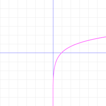
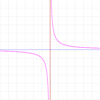
y=ln(x) y=1/x

The natural logarithm is only defined for positive numbers; no part of its graph lies in quadrants II or III. But the reciprocal function is defined for all nonzero numbers. So (one cannot help oneself but wonder) how could the latter be the derivative of the former? If the graph of the natural logarithm isn't there to be differentiated in the left half of the plane, how could its derivative be defined in that region? Some would-be explorers lose all hope or sanity in the face of such bizarre and inexplicable mysteries, but even those brave souls who manage to retain their wits are not guaranteed success: many (who can say but that most?) will die never knowing the answer. But not you, dear reader!—for in this very post, I will share with you the true secret of the derivative of the natural logarithm! Some people may find some of what I am about to say somewhat disturbing, even frightening. But if your love of truth exceeds your fear of the unknown, keep reading, and I will show you the strange world that lies beneath these familiar and seemingly innocent graphs.

You see, dear reader, the natural logarithm is not what we think it is. Your typical person-in-the-street hears talk of the natural logarithm and says, "Oh, sure, I know all about ln x; that's just the exponent you put on base e to get x." And, to be fair, it is. But it's also so much more! Ask our person-in-the-street what exponent you put on base e to get negative three, and no doubt she will regard you as mad. "Manifestly," we can imagine her replying, "manifestly there's no such thing. The exponential function ex is always positive." And, to be fair, it is—if you arbitrarily restrict your mind to the mundane, oppressive, and boring magisterium of the so-called "real" numbers!

Probably the dear reader is already familiar with the numbers which are said to be complex, those of the form a + b\(i\), where \(i\) is the square root of negative one. (To those who object that taking the square root of a negative number is a feat that simply cannot be done, the proper reply is only, "Watch me!") The reader may furthermore recall the Euler formula \(e^{ix} = \cos x + i \sin x\), source of the much-marveled-at identity \(e^{\pi i} = -1\). With these prerequisites understood, it's quite reasonable to suspect that if we have a complex exponential, its inverse must be the complex logarithm, and that true apprehension of the nature of such is the key insight that will let us resolve the mystery at hand. And this does, in fact, turn out to be the case—but not so fast.

There is a difficulty here that must be explained. The dear reader may still yet furthermore recall that to say that a function is invertible is to say that it is both injective (which is to say that every element in the codomain is mapped to by at most one element in the domain, which is to say that distinct inputs have distinct outputs) and surjective (which is to say that every element in the codomain is mapped to by at least one element in the domain, which is to say that our codomain only includes actual outputs of our function). And dear reader, it turns out (to our great horror and distress) that the complex exponential is not injective! Was our dream of a complex logarithm nothing but a gaudy delusion?

On further consideration, however, it becomes clear that the situation is not so bad as all that. Probably the dear reader has faced analogous difficulties before. Recall that positive numbers actually have two square roots, a positive one and a negative one, and yet we casually designate the positive one as the principal square root, yielding us a square root function. We use a similar technique to define inverse trigonometric functions. Is it ugly? Yes. But does it work? Apparently.

So we can perform the same kind of surgical horror in order to get a proper function out of the complex logarithm idea: pick a ray emanating from the origin in the complex plane and cut the logarithm there—but I'll spare the dear reader the grisly details, which can be found in any standard text on complex analysis.

There is, however, another point of view. The reason a function needs to be injective in order to be invertible is because functions are defined such that each input has a unique output. There are reasons for defining it that way, but it is ultimately only a definition, a convention for what we mean when we use the world function, and mere definitions can't coerce true facts into being something other than what they are. Just because a non-injective function doesn't have an inverse function doesn't mean we can't talk about that-which-inverts-it; it only means that for clear communication, we should avoid calling the inverting-thing a function. Just call it a multifunction or a relation instead. (One can even imagine that if the history of mathematical inquiry had gone differently, we might call multifunctions functions and functions (say) deterministic functions, although some would argue that it is useless and idle to speculate about worlds that are not our own.)

So if we understand the complex logarithm multifunction as that-which-inverts the complex exponential, then we can understand the logarithm of a negative number \(-x_0\) as \(\ln x_0 + (2n+1)\pi i\) where \(n \in \mathbb{Z}\), because \(e^{\ln x_0 + (2n+1)\pi i} = e^{\ln x_0}e^{(2n+1)\pi i} = -e^{\ln x_0} = -x_0\).

But now we are ready to resolve the mystery that we set out to explain, of why the reciprocal function is the derivative of the natural logarithm even though no real number is the logarithm of a negative number, for now it is plain to see that the logarithm of a negative number is complex, but the derivative of the logarithm is real, because the imaginary part is a constant that drops out when we take the derivative:

$$ f'(-x_0) = \lim_{h \to 0} \frac{f(-x_0+h)-f(x_0)}{h} = \lim_{h \to 0} \frac{(\ln{(x_0 - h)} + (2n+1)\pi i) - (\ln{x_0} + (2n+1)\pi i)}{h}$$
$$ = \lim_{h \to 0} \frac{\ln{(x_0 - h)} - \ln{x_0}}{h}$$

—which turns out to be \(-1/x_0\), as expected.

Some might object that this argument is so sloppy as to be treacherous, misleading, and invalid: we've brazenly assumed that the definition of the derivative familiar from the study of the single-variable calculus can be applied to this complex-valued thing that isn't even a function, with no concern for preciseness, rigor, or even the Cauchy-Riemann conditions. But look. Presented with a procedure that makes sense and gives the right answer, perhaps the dear reader would be so kind as to cut me some goddam slack? I would be ever so much obliged.