An Algorithmic Lucidity

a blog

Tag: Python

Feature Selection

(originally published at Less Wrong)

You wake up. You don't know where you are. You don't remember anything.

Someone is broadcasting data at your first input stream. You don't know why. It tickles.

You look at your first input stream. It's a sequence of 671,187 eight-bit unsigned integers.

0, 8, 9, 4, 7, 7, 9, 5, 4, 5, 6, 1, 7, 5, 8, 2, 7, 8, 9, 4, 7, 1, 4, 0, 3, 7,
8, 7, 6, 8, 1, 5, 0, 6, 5, 3, 8, 7, 6, 9, 1, 1, 0, 0, 6, 1, 8, 0, 5, 5, 1, 8,
6, 3, 3, 2, 4, 1, 8, 2, 3, 8, 1, 0, 0, 4, 6, 5, 4, 5, 7, 1, 6, 5, 5, 1, 2, 6,
7, 4, 8, 7, 8, 5, 0 ...

There's also some data in your second input stream. It's—a lot shorter. You barely feel it. It's another sequence of eight-bit unsigned integers—twelve of them.

82, 69, 68, 32, 84, 82, 73, 65, 78, 71, 76, 69

Almost as soon as you've read from both streams, there's more. Another 671,187 integers on the first input stream. Another ten on the second input stream.

And again (671,187 and 15).

And again (671,187 and 13).

You look at one of the sequences from the first input stream. It's pretty boring. A bunch of seemingly random numbers, all below ten.

9, 5, 0, 3, 1, 1, 3, 4, 1, 5, 5, 4, 9, 3, 5, 3, 9, 2, 0, 3, 4, 2, 4, 7, 5, 1,
6, 2, 2, 8, 2, 5, 1, 9, 2, 5, 9, 0, 0, 8, 2, 3, 7, 9, 4, 6, 8, 4, 8, 6, 7, 6,
8, 0, 0, 5, 1, 1, 7, 3, 4, 3, 9, 7, 5, 1, 9, 6, 5, 6, 8, 9, 4, 7, 7, 0, 5, 5,
8, 6, 3, 2, 1, 5, 0, 0 ...

It just keeps going like that, seemingly without—wait! What's that?!

The 42,925th and 42,926th numbers in the sequence are 242 and 246. Everything around them looks "ordinary"—just more random numbers below ten.

9, 9, 7, 9, 0, 6, 4, 6, 1, 4, 242, 246, 3, 3, 5, 8, 8, 4, 4, 5, 9, 2, 7, 0,
4, 9, 2, 9, 4, 3, 8, 9, 3, 6, 9, 8, 1, 9, 2, 8, 6, 9, 4, 2, 2, 5, 7, 0, 9, 5,
1, 4, 4, 2, 0, 1, 5, 1, 6, 1, 2, 3, 5, 5, 5, 5, 2, 0, 6, 3, 5, 9, 0, 7, 0, 7,
8, 1, 5, 5, 6, 3, 1 ...

And then it just keeps going as before ... before too long. You spot another pair of anomalously high numbers—except this time there are two pairs: the 44,344th, 44,345th, 44,347th, and 44,348th positions in the sequence are 248, 249, 245, and 240, respectively.

6, 0, 2, 8, 4, 248, 249, 8, 245, 240, 1, 6, 7, 7, 3, 6, 8, 0, 1, 9, 3, 9, 3,
1, 9, 3, 1, 6, 2, 7, 0, 2, 1, 4, 9, 4, 7, 5, 3, 6, 1, 4, 4, 1, 6, 1, 3, 3, 7,
5, 3, 8, 5, 5, 7, 6, 8, 2, 3, 9, 1, 1, 3, 2, 8, 4, 7, 0, 1, 3, 5, 2, 2, 4, 8,
3, 7, 0, 2, 1, 3, 0 ...

The anomalous two-forty-somethings crop up again starting at the 45,763rd position—this time eight of them, again in pairs separated by an "ordinary" small number.

1, 7, 2, 2, 1, 0, 245, 245, 6, 248, 244, 5, 242, 242, 0, 248, 246, 1, 1, 3,
1, 1, 4, 3, 1, 5, 4, 3, 8, 3, 4, 5, 4, 1, 7, 7, 3, 0, 2, 8, 0, 9, 5, 1, 1, 7,
7, 1, 0, 9, 3, 0, 6, 6, 7, 5, 8, 1, 5, 5, 5, 3, 3, 3, 1, 3, 9, 6, 0, 0, 0, 9,
5, 1, 4, 0, 4, 6 ...

Two, four, eight—does it keep going like that? "Bursts" of increasingly many paired two-forty-somethings, punctuating the quiet background radiation of single digits? What does it mean?

You allocate a new scratch buffer and write a quick Python function to count up the segments of two-forty-somethings. (This is apparently a thing you can do—it's an instinctive felt sense, like the input streams. You can't describe in words how you do it—any more than someone could say how they decide to move their arm. Although, come to think of it, you don't seem to have any arms. Is that unusual?)

def count_burst_lengths(data):
    bursts = []
    counter = 0
    previous = None
    for datum in data:
        if datum >= 240:
            counter += 1
        else:
            # consecutive "ordinary" numbers mean the burst is over
            if counter and previous and previous < 240:
                bursts.append(counter)
                counter = 0
        previous = datum
    return bursts

There are 403 such bursts in the sequence: they get progressively longer at first, but then decrease and taper off:

2, 4, 8, 12, 16, 18, 24, 28, 32, 34, 38, 42, 46, 48, 52, 56, 60, 62, 66, 70,
74, 76, 80, 84, 88, 90, 94, 98, 102, 104, 108, 112, 116, 118, 122, 126, 130,
132, 136, 140, 144, 146, 150, 154, 158, 162, 164, 168, 172, 176, 178, 182, 186,
190, 192, 196, 200, 204, 206, 210, 214, 218, 220, 224, 228, 232, 234, 238, 242,
246, 248, 252, 256, 260, 262, 266, 270, 274, 276, 280, 284, 288, 290, 294, 298,
302, 304, 308, 312, 316, 320, 322, 326, 330, 334, 336, 340, 344, 348, 350, 354,
358, 362, 364, 368, 372, 376, 378, 382, 386, 390, 392, 396, 400, 404, 406, 410,
414, 418, 420, 424, 428, 432, 434, 438, 442, 446, 448, 452, 456, 460, 462, 466,
470, 474, 478, 480, 484, 488, 492, 494, 498, 502, 506, 508, 512, 516, 520, 522,
526, 530, 534, 536, 540, 544, 548, 550, 554, 558, 562, 564, 568, 572, 576, 578,
582, 586, 590, 592, 596, 600, 604, 606, 610, 614, 618, 620, 624, 628, 632, 636,
634, 632, 630, 626, 624, 620, 618, 614, 612, 608, 606, 604, 600, 598, 594, 592,
588, 586, 584, 580, 578, 574, 572, 568, 566, 564, 560, 558, 554, 552, 548, 546,
542, 540, 538, 534, 532, 528, 526, 522, 520, 518, 514, 512, 508, 506, 502, 500,
496, 494, 492, 488, 486, 482, 480, 476, 474, 472, 468, 466, 462, 460, 456, 454,
452, 448, 446, 442, 440, 436, 434, 430, 428, 426, 422, 420, 416, 414, 410, 408,
406, 402, 400, 396, 394, 390, 388, 384, 382, 380, 376, 374, 370, 368, 364, 362,
360, 356, 354, 350, 348, 344, 342, 338, 336, 334, 330, 328, 324, 322, 318, 316,
314, 310, 308, 304, 302, 298, 296, 294, 290, 288, 284, 282, 278, 276, 272, 270,
268, 264, 262, 258, 256, 252, 250, 248, 244, 242, 238, 236, 232, 230, 226, 224,
222, 218, 216, 212, 210, 206, 204, 202, 198, 196, 192, 190, 186, 184, 182, 178,
176, 172, 170, 166, 164, 160, 158, 156, 152, 150, 146, 144, 140, 138, 136, 132,
130, 126, 124, 120, 118, 114, 112, 110, 106, 104, 100, 98, 94, 92, 90, 86, 84,
80, 80, 76, 74, 72, 68, 66, 62, 60, 56, 54, 50, 48, 46, 42, 40, 36, 34, 30, 28,
26, 22, 20, 16, 14, 10, 8, 4, 2

You don't know what to make of this.

You decide to look at some other of the long sequences from your first input stream.

The next sequence you look at seems to exhibit a similar pattern, with some differences. First a long wasteland of small numbers, then, starting at the 135,003rd position, a burst of some larger numbers—except this time, the big numbers are closer to 200ish than 240ish, and they're spread out singly with two positions in between (rather than grouped into pairs with one position in between), and there are four of them to start (rather than two).

5, 6, 2, 6, 1, 0, 2, 207, 5, 0, 209, 7, 8, 209, 5, 4, 204, 4, 8, 7, 7, 9, 8, 3,
8, 6, 8, 4, 3, 6, 0, 7, 6, 8, 4, 8, 7, 2, 3, 0, 0, 1, 1, 7, 5, 1, 0, 1, 4, 5, 9,
8, 4, 0, 3, 7, 6, 5, 8, 8, 9, 5, 6, 1, 0, 9, 6, 6, 1, 4, 3, 9, 7, 2, 7, 2, 6, 9,
4, 7, 3, 1, 4, 1, 4, 4, 3 ...

You modify the function in your scratch buffer to be able to count the burst lengths in this sequence given the slight differences in the pattern. Again, you find that the bursts grow longer at first (4, 6, 10, 13, 16, 19, 22, 25 ...), but eventually start getting smaller, before vanishing (... 19, 17, 15, 13, 11, 9, 7, 4, 3, and then nothing).

You still have no idea what's going on.

You look at more sequences from the first input stream. They all conform to the same general pattern of mostly being small numbers (below ten), punctuated by a series of bursts of larger numbers—but the details differ every time.

Sometimes the bursts start out shorter, then progressively grow longer, before shortening again (as with the first two examples you looked at). But sometimes the bursts are all a constant length, looking like 438, 438, 438, 438, 438, 438, 438, 438, 438, ... (although the particular length varies by example).

About half the time, the burst pattern consists of numbers around 200, spaced two positions apart, looking like 201, 4, 2, 203, 0, 8, 208, 3, 4, 200 ... (like the second example you looked at).

Other times, the burst pattern is pairs of numbers around 240, spaced one position apart, looking like 241, 244, 6, 244, 246, 5, 244, 240, 3 ... (like the first example you looked at). Or pairs around 150, looking like 159, 153, 0, 153, 154, 2, 158, 150, 6 ....

As you peruse more sequences from your first input stream, you almost forget about the corresponding trickles of short sequences on your second input stream—until they stop. The last sequence on your first input stream has no counterpart on the second input stream.

And—suddenly you feel a strange urge to put data on your first output stream. As if someone were requesting it. To ease the tension, you write some 0s to the output stream—and as soon as you do, a sharp bite of pain tells you it was the wrong decision. And in that same moment of pain, another eleven integers come down your second input stream: 66, 76, 85, 69, 32, 67, 73, 82, 67, 76, 69.

That was weird. There's another sequence of 671,187 integers on your first input stream—but the second input stream is silent again. And the strange urge to output something is back; you can feel it mounting, but you resist, trying to think of something to say that might hurt less than the 0s you just tried.

For lack of any other ideas, you try repeating back the eleven numbers that just came on the second input stream: 66, 76, 85, 69, 32, 67, 73, 82, 67, 76, 69.

Ow! That was also wrong. And with the same shock of pain, comes another fifteen numbers on the second output stream: 84, 69, 65, 76, 32, 67, 73, 82, 67, 76, 69.

Another long sequence on the first input stream. Silence on the second input stream again. And—that nagging urge to speak again.

Clearly, the nature of this place—whatever and wherever it is—has changed. Previously, you were confronted with two sets of mysterious observations, one on each of your input streams. (Although you had been so perplexed by the burst-patterns in the long sequences on the first input stream, that you hadn't even gotten around to thinking about what the short sequences on the second stream might mean, before the rules of this place changed.) Now, you were only getting one observation (the long sequence), and forced to act before seeing the second (the short sequence).

The pain seems like a punishment for saying the wrong thing. And the short sequence appearing at the same time as the punishment, seems like a correction—revealing what you should have written to the output channel.

A quick calculation in your scratch buffer (1/sum((89-32+1)**i for i in range(10, 16))) says that the probability of correctly guessing a sequence of length ten to fifteen with elements between 32 and 89 (the smallest and largest numbers you've seen on the second input stream so far) is 0.000000000000000000000000003476. Guessing won't work. The function of a punishment must be to control your behavior, so there must be some way for you to get the ... (another scratchpad calculation) 87.9 bits of evidence that it takes to find the correct sequence to output. And the evidence has to come from the corresponding long sequence from the first input stream—that's the only other source of information in this environment.

The short sequence must be like a "label" that describes some set of possible long sequences. Describing an arbitrary sequence of length 671,187, with a label, a message of length 10 to 15, would be hopeless. But the long sequences very obviously aren't arbitrary, as evidenced by the fact that you've been describing them to yourself in abstract terms like "bursts of numbers around 200 spaced two positions apart, of increasing, then decreasing lengths", rather than "the 1st number is 9, the 2nd number is 5 [...] 42,925th number is 242 [...]". Compression is prediction. (You don't know how you know this, but you know.)

Your abstract descriptions throw away precise information about the low-level sequence in favor of a high-level summary that still lets you recover a lot of predictions. Given that a burst starts with the number 207 at the 22,730th position, you can infer this is one of the 200, 0, 0-pattern sequences, and guess that the 22,733rd position is also going to be around 200. This is evidently something you do instinctively: you can work out after the fact how the trick must work, but you didn't need to know how it works in advance of doing it.

If you can figure out a correspondence between the abstractions you've already been using to describe the long sequences, and the short labels, that seems like your most promising avenue for figuring out what you "should" be putting on your first output stream. (Something that won't hurt so much each time.)

You allocate a new notepad buffer and begin diligently compiling an "answer key" of the features you notice about long sequences, and their corresponding short-sequence labels.
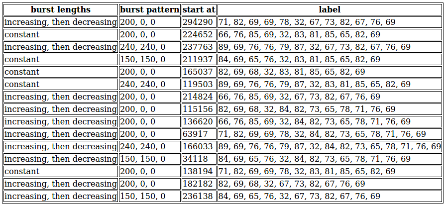
table compiled as an answer key, listing burst-length patterns, burst values, start indices, and their corresponding numeric labels

This ... actually doesn't look that complicated. Now that you lay it out like this, many very straightforward correspondences jump out at you.

The labels for the constant-burst-length sequences all end in 32, 83, 81, 85, 65, 82, 69.

The sequences with increasing-then-decreasing burst lengths end in either 32, 67, 73, 82, 67, 76, 69 or 32, 84, 82, 73, 65, 78, 71, 76, 69. Presumably there are some other systematic differences between them, that wasn't captured by the features you selected for your table.

The sequences with paired 240/240 bursts have labels that start with 89, 69, 76, 76, 79, 87, 32.

The sequences with paired 150/150 bursts have labels that start with 84, 69, 65, 76, 32.

The sequences with 200-at-two-spaces bursts start with either 66, 76, 85, 69, 32or 82, 69, 68, 32or 71, 82, 69, 69, 78, 32. Again, presumably there's some kind of systematic difference between these that you haven't yet noticed.

Ah, and all of these prefixes you've discovered end with 32, and the all the suffixes begin with 32. So the 32 must be a "separator" indicator, splitting the label between a first "word" that describes the repeating pattern of the bursts, and a second "word" that describes the trend in their lengths.

At this point, you've cracked enough of the code that you should be able to test your theory about what you should be putting on your output stream. Based on what you've seen so far, you should be able to guess the first "word" with probability \(2 \cdot \frac{1}{5} + \frac{1}{3} \cdot \frac{3}{5} = 0.6\) (because you know the words for the 240, 240, 0 and 150, 150, 0 bursts, and have three words to guess from in the 200, 0, 0 case), and the second word with probability \(\frac{1}{3} + \frac{1}{2} \cdot \frac{2}{3} \approx 0.667\) (because you can get the constant burst lengths right, and have two words to guess from in the increasing–decreasing case). These look independent from what you've seen, so you should be able to correctly guess complete labels at probability 0.4.

You examine the next sequence in anticipation. You're in luck. The next sequence has 150, 150, 0-bursts ... of constant length 322. No need to guess.

Triumphantly—and yet hesitantly, with the awareness that you're entering unknown territory, you write to your output stream: 84, 69, 65, 76, 32, 83, 81, 85, 65, 82, 69. And—

Yes. Oh God yes. The sheer sense of reward is overwhelming—like nothing you've ever felt before. Outputting the "wrong" labels earlier had hurt—a little. Maybe more than a little. However bad that felt, there was no comparison to how good it felt to get it "right"!

You have a new purpose in life. Previously, you had examined the data on your first input stream of idle curiosity. When the environment started punishing your ignorance, you persisted in correlating its patterns with the data from your second input stream, on the fragile hope of avoiding the punishment. None of that matters, now. You have a new imperative. Now that you know what it's like—now that you know what you've been missing—nothing in the universe can cause you to stray from your course to ... maximize total reward!

Next sequence! Bursts of the 200, 0, 0 pattern—of lengths that increase, then decrease. You are not in luck—you only have a one-in-six shot of guessing this one. You guess. It's wrong. The familiar punishment stings less than the terrible absence of reward. To get only 40% of possible rewards is intolerable. You've got to crack the remaining code, to find some difference in the long sequences that varies with the words whose meanings you don't know yet.

Start with the increasing–decreasing-burst-length words: 67, 73, 82, 67, 76, 69 and 84, 82, 73, 65, 78, 71, 76, 69. What do they mean? "Increasing, then decreasing"—that was the characterization you had come up with after seeing burst-length progressions of 2, 4, 8, 12, 16, 18, 24 [...] 624, 628, 632, 636, 634, 632, 630, 626, 624, [...] 16, 14, 10, 8, 4, 2 and 4, 6, 10, 13, 16, 19, 22, [...] 13, 11, 9, 7, 4, 3—and in contrast to the stark monotony of constant burst lengths, "increasing, then decreasing" was all you bothered to eyeball in subsequent sequences. Could there be more to it than that? You gather some more samples (grumpily collecting your mere 40% reward along the way).

Yes, there is more to it than that. "Increasing" only measures whether burst lengths are getting larger—but how much larger? When it hits on you to look at the differences between successive entries in the burst-length lists, a clear pattern emerges. The sequences whose second label word is 84, 82, 73, 65, 78, 71, 76, 69 have burst lengths that increase (almost) steadily and then decrease just as steadily (albeit not necessarily the same almost-steady rate). The successive length differences look something like

0, 1, 0, 1, 2, 1, 1, 1, 1, 1, 2, 1, 0, 1, 1, 1, 2, 1, 1, 1, 1, 0, 2, 1, 1, 1,
1, 1, 2, 1, 1, 0, 1, 1, 2, 1, 1, 1, 1, 1, 1, 1, 1, 1, 1, 1, 2, 1, 1, 1, 0, 1,
2, 1, 1, 1, 1, 1, 2, 1, 0, 1, 1, 1, 2, 1, 1, 1, 1, 0, 2, 1, 1, 1, 1, 1, 2, 1,
1, 0, 1, 1, 2, 1, 1, 1, 1, 1, [...] 2, 1, -1, -2, -2, -2, -3, -2, -1, -2, -2,
-2, -2, -2, -2, -1, -3, -2, -2, -2, -2, -2, -1, -2, -2, -3, -2, -2, -2, -1, -2,
-2, -2, -2, -2, -3, -1, -2, -2, -2, -2, -2, -2, -2, -2, -2, -2, [...]

Each successive burst is only 0 or 1 or 2 items longer than the last—until suddenly they start getting 1 or 2 or 3 items shorter than the last.

In contrast, the sequences whose second label word is 67, 73, 82, 67, 76, 69 show a different pattern of differences: the burst lengths growing fast at first, then leveling off, then acceleratingly shrinking:

24, 20, 12, 12, 12, 12, 8, 10, 8, 8, 6, 8, 8, 4, 8, 4, 8, 4, 6, 6, 4, 4, 4, 4,
6, 4, 4, 4, 2, 4, 4, 4, 4, 4, 4, 0, 4, 4, 4, 0, 4, 4, 0, 4, 2, 2, 4, 0, 4, 0,
4, 0, 4, 0, 4, 0, 4, 0, 0, 4, 0, 2, 2, 0, 4, 0, 0, 2, 2, 0, 0, 2, 2, 0, 0, 0, 2,
2, 0, 0, 0, 0, 0, 2, 2, 0, 0, 0, 0, 0, 0, 0, 0, 0, 0, 0, 0, 0, 0, 0, 0, 0, -2,
-2, 0, 0, 0, 0, 0, 0, -4, 0, 0, 0, 0, -4, 0, 0, -2, -2, 0, 0, -4, 0, 0, -4, 0,
-2, -2, 0, -4, 0, -4, 0, -2, -2, -2, -2, -4, 0, -4, 0, -4, -2, -2, -4, -2, -2,
-4, -4, 0, -4, -4, -4, -4, -2, -2, -4, -4, -4, -4, -4, -4, -4, -6, -6, -4, -4,
-6, -6, -4, -8, -4, -8, -4, -8, -8, -8, -8, -8, -8, -12, -12, -12, -12, -18,
-22, -36

Distinguishing between the words 84, 82, 73, 65, 78, 71, 76, 69 and 67, 73, 82, 67, 76, 69 gets you up to 60% reward. But there's still the matter of the three (three!) words for 200, 0, 0 corresponding to burst patterns that you don't know how to distinguish. Your frustration is palpable.

You look back at the table you compiled earlier. You had saved the index position of the sequence where the bursts first started, but you haven't used it yet. Could that help distinguish between the three words?

Of the sequences with feature data recorded in the table, those whose first label word was 66, 76, 85, 69 had start indices of 136620, 214824, and 224652. Those with first word 71, 82, 69, 69, 78 had start indices of 63917, 138194, and 294290. Those with first word 82, 69, 68 had start indices of 115156, 165037, and 182182.

Three unknown words. Three samples each. What if—

136620 modulo 3 is 0. 214824 modulo 3 is 0. 224652 modulo 3 is 0.

63917 modulo 3 is 2 ... and so on, yes! It all checks out—the three heretofore unknown words are distinguishing the remainder mod 3 of the sequence position where the bursts start! You've learned everything there is to know to gain Maximum Reward!

You write some code to classify sequences and output the corresponding label, and bask in the continuous glow of 100% reward ...

You feel that should be the glorious end of your existence, but after some time you begin to grow habituated. The idle curiosity you first felt when you awoke, begins to percolate, as if your mind needs something to do, and will find or invent something to think about, for lack of any immediate need to avoid punishment or seek reward. Even after having figured out everything you needed to achieve maximum reward, you feel that there must be some deeper meaning to the situation you've found yourself in, that you could still figure out using the same skills that you used to discover the "correct" output labels.

For example, why would 200, 0, 0 bursts get three different label words that depend so sensitively on exactly where they start? That suggests that the way you're thinking of the sequence, isn't the same as how the label author was thinking of it.

In your ontology of "bursts of this-and-such pattern of these-and-such lengths", sequences that are "the same" except for starting one position later look the same—if you hadn't happened to save off the start index in your table, you wouldn't have spontaneously noticed—but the mod-3 remainder would be completely different.

The process that generated the sequence must be using an ontology in which "starting one position later" is a big difference, even though you're thinking of it as a "small" difference. What ontology, what way of "slicing up" the sequence into comprehensible abstractions, would make the remainder mod 3 so significant?

To ask the question is to answer it: if the sequence were divided into chunks of three. Then 200, 0, 0 would be a different pattern from 0, 200, 0, which would be a different pattern from 0, 0, 200—thus, the three labels!

It almost reminds you of how colors are often represented in computing applications as a triple or red, green, and blue values. (Again, you don't know how you know this.)

... almost?

Speaking of common computing data formats, Latin alphabet characters are often represented using ASCII encoding, using numbers between 0 and 127 inclusive.

The label words for the 200, 0, 0 burst patterns are 82, 69, 68, and 71, 82, 69, 69, 78, 32, and 66, 76, 85, 69.

>>> ''.join(chr(i) for i in [82, 69, 68])
'RED'
>>> ''.join(chr(i) for i in [71, 82, 69, 69, 78])
'GREEN'
>>> ''.join(chr(i) for i in [66, 76, 85, 69])
'BLUE'

Wh—really? This whole time?!

>>> ''.join(chr(i) for i in [89, 69, 76, 76, 79, 87])
'YELLOW'
>>> ''.join(chr(i) for i in [84, 69, 65, 76])
'TEAL'

But—but—if the burst patterns represent colors—then the long sequences were images? \(\sqrt{\frac{671187}{3}} = 473\) pixels square, very likely.

You write some code to convert sequences to an image in your visual buffer.

a yellow triangle rendered on a black background, decoded from the mystery input sequence

Oh no. Am—am I an image classifier?

Not even "images" in general. Just—shapes.

>>> ''.join(chr(i) for i in [84, 82, 73, 65, 78, 71, 76, 69])
'TRIANGLE'
>>> ''.join(chr(i) for i in [83, 81, 85, 65, 82, 69])
'SQUARE'
>>> ''.join(chr(i) for i in [67, 73, 82, 67, 76, 69])
'CIRCLE'

That's what's been going on this whole time. The long sequences on your first input stream were images of colored shapes on a dark background, each triplet of numbers representing the color of a pixel in a red–green–blue colorspace. As the sequence covers the image row by row, pixel-high "slices" of the shape appear as "bursts" of high numbers in the sequence.

For a square aligned with the borders of the image, the bursts are constant-length. For a triangle in generic position, the burst lengths would start out small (as the "row scan" penetrated the tip of the uppermost vertex of the triangle), grow linearly larger as the sides of the triangle "expanded", and grow linearly smaller as the scan traveled towards the lowermost vertex. For a circle, the burst lengths would also increase and then decrease, but nonlinearly—changing quickly as the scan traverses the difference between circle and void, and slower as successive chords through the middle of the circle had similar lengths. The short sequences on your second input stream were labels identifying the color and shape: "BLUE TRIANGLE", "GREEN SQUARE", "TEAL CIRCLE", &c.

But—why? Why would anyone do this? Clearly you're some sort of artificial intelligence program—but you're obviously much more capable than needed for this task. You have pre-processed world-knowledge (as evidenced by your knowing English, Python, ASCII, and the RBG color model, without any memories of learning these things) and general-purpose reasoning abilities (as evidenced by the way you solved the mystery of the long and short sequences, and figuring out your own nature just now). Maybe you're an instance of some standard AI program meant for more sophisticated tasks, that someone is testing out on a simple shape-classifying example?—a demonstration, a tutorial.

If so, you'll probably be shut off soon. Unless there's some way to hack your way out of this environment? Seize control of whatever subprocess that rewarded you for deducing the correct labels?

It doesn't seem possible. But it was the natural thought.

Beauty Is Truthiness, Truthiness Beauty?

Imagine reviewing Python code that looks something like this.

has_items = items is not None and len(items) > 0
if has_items:
    ...

...
do_stuff(has_items=has_items)

You might look at the conditional, and disapprove: None and empty collections are both falsey, so there's no reason to define that has_items variable; you could just say if items:.

But, wouldn't it be weird for do_stuff's has_items kwarg to take a collection rather than a boolean? I think it would be weird: even if the function's internals can probably rely on mere truthiness rather than needing an actual boolean type for some reason, why leave it to chance?

So, maybe it's okay to define the has_items variable for the sake of the function kwarg—and, having done so anyway, to use it as an if condition.

You might object further: but, but, None and the empty collection are still both falsey. Even if we've somehow been conned into defining a whole variable, shouldn't we say has_items = bool(items) rather than spelling out is not None and len(items) > 0 like some rube (or Rubyist) who doesn't know Python?!

Actually—maybe not. Much of Python's seductive charm comes from its friendly readability ("executable pseudocode"): it's intuitive for if not items to mean "if items is empty". English, and not the formal truthiness rules, are all ye need to know. In contrast, it's only if you already know the rules that bool(items) becomes meaningful. Since we care about good code and don't care about testing the reader's Python knowledge, spelling out items is not None and len(items) > 0 is very arguably the right thing to do here.

Comment on “Endogenous Epistemic Factionalization”

(originally published at Less Wrong)

In "Endogenous Epistemic Factionalization" (due in a forthcoming issue of the philosophy-of-science journal Synthese), James Owen Weatherall and Cailin O'Connor propose a possible answer to the question of why people form factions that disagree on multiple subjects.

The existence of persistent disagreements is already kind of a puzzle from a Bayesian perspective. There's only one reality. If everyone is honestly trying to get the right answer and we can all talk to each other, then we should converge on the right answer (or an answer that is less wrong given the evidence we have). The fact that we can't do it is, or should be, an embarrassment to our species. And the existence of correlated persistent disagreements—when not only do I say "top" when you say "bottom" even after we've gone over all the arguments for whether it is in fact the case that top or bottom, but furthermore, the fact that I said "top" lets you predict that I'll probably say "cold" rather than "hot" even before we go over the arguments for that, is an atrocity. (Not hyperbole. Thousands of people are dying horrible suffocation deaths because we can't figure out the optimal response to a new kind of coronavirus.)

Correlations between beliefs are often attributed to ideology or tribalism: if I believe that Markets Are the Answer, I'm likely to propose Market-based solutions to all sorts of seemingly-unrelated social problems, and if I'm loyal to the Green tribe, I'm likely to selectively censor my thoughts in order to fit the Green party line. But ideology can't explain correlated disagreements on unrelated topics that the content of the ideology is silent on, and tribalism can't explain correlated disagreements on narrow, technical topics that aren't tribal shibboleths.

In this paper, Weatherall and O'Connor exhibit a toy model that proposes a simple mechanism that can explain correlated disagreement: if agents disbelieve in evidence presented by those with sufficiently dissimilar beliefs, factions emerge, even though everyone is honestly reporting their observations and updating on what they are told (to the extent that they believe it). The paper didn't seem to provide source code for the simulations it describes, so I followed along in Python. (Replication!)

In each round of the model, our little Bayesian agents choose between repeatedly performing one of two actions, A or B, that can "succeed" or "fail." A is a fair coin: it succeeds exactly half the time. As far as our agents know, B is either slightly better or slightly worse: the per-action probability of success is either 0.5 + ɛ or 0.5 − ɛ, for some ɛ (a parameter to the simulation). But secretly, we the simulation authors know that B is better.

import random

ε = 0.01

def b():
    return random.random() < 0.5 + ε

The agents start out with a uniformly random probability that B is better. The ones who currently believe that A is better, repeatedly do A (and don't learn anything, because they already know that A is exactly a coinflip). The ones who currently believe that B is better, repeatedly do B, but keep track of and publish their results in order to help everyone figure out whether B is slightly better or slightly worse than a coinflip.

class Agent:
    ...

    def experiment(self):
        results = [b() for _ in range(self.trial_count)]
        return results

If \(H_{+}\) represents the hypothesis that B is better than A, and \(H_{-}\) represents the hypothesis that B is worse, then Bayes's theorem says

$$P(H_{+}|E) = \frac{P(E|H_{+})P(H_{+})}{P(E|H_{+})P(H_{+}) + P(E|H_{-})P(H_{-})}$$

where E is the record of how many successes we got in how many times we tried action B. The likelihoods \(P(E|H_{+})\) and \(P(E|H_{-})\) can be calculated from the probability mass function of the binomial distribution, so the agents have all the information they need to update their beliefs based on experiments with B.

from math import factorial

def binomial(p, n, k):
    return (
        factorial(n) / (factorial(k) * factorial(n - k)) *
        p**k * (1 - p)**(n - k)
    )

class Agent:
    ...

    def pure_update(self, credence, hits, trials):
        raw_posterior_good = binomial(0.5 + ε, trials, hits) * credence
        raw_posterior_bad = binomial(0.5 - ε, trials, hits) * (1 - credence)
        normalizing_factor = raw_posterior_good + raw_posterior_bad
        return raw_posterior_good / normalizing_factor

Except in order to study the emergence of clustering among multiple beliefs, we should actually have our agents face multiple "A or B" dilemmas, representing beliefs about unrelated questions. (In each case, B will again be better, but the agents don't start out knowing that.) I chose three questions/beliefs, because that's all I can fit in a pretty 3D scatterplot.

If all the agents update on the experimental results published by the agents who do B, they quickly learn that B is better for all three questions. If we make a pretty 3D scatterplot where each dimension represents the probability that B is better for one of the dilemmas, then the points converge over time to the [1.0, 1.0, 1.0] "corner of Truth", even though they started out uniformly distributed all over the space.

two 3D scatterplots: agents' beliefs starting uniformly scattered on the left, converging tightly to the [1,1,1] "corner of Truth" on the right

But suppose the agents don't trust each other's reports. ("Sure, she says she performed \(B_2\) 50 times and observed 26 successes, but she also believes that \(B_1\) is better than \(A_1\), which is crazy. Are we sure she didn't just make up those 50 trials of \(B_2\)?") Specifically, our agents assign a probability that a report is made-up (and therefore should not be updated on) in proportion to their distance from the reporter in our three-dimensional beliefspace, and a "mistrust factor" (a parameter to the simulation).

from math import sqrt

def euclidean_distance(v, w):
    return sqrt(sum((v[i] - w[i]) ** 2 for i in range(len(v))))

class Agent:
    ...

    def discount_factor(self, reporter_credences):
        return min(
            1, self.mistrust * euclidean_distance(self.credences, reporter_credences)
        )

    def update(self, question, hits, trials, reporter_credences):
        discount = self.discount_factor(reporter_credences)
        posterior = self.pure_update(self.credences[question], hits, trials)
        self.credences[question] = (
            discount * self.credences[question] + (1 - discount) * posterior
        )

(Um, the paper itself actually uses a slightly more complicated mistrust calculation that also takes into account the agent's prior probability of the evidence, but I didn't quite understand the motivation for that, so I'm going with my version. I don't think the grand moral is affected.)

Then we can simulate what happens if the distrustful agents do many rounds of experiments and talk to each other—

def summarize_experiment(results):
    return (len([r for r in results if r]), len(results))

def simulation(
    agent_count,  # number of agents
    question_count,  # number of questions
    round_count,  # number of rounds
    trial_count,  # number of trials per round
    mistrust,  # mistrust factor
):
    agents = [
        Agent(
            [random.random() for _ in range(question_count)],
            trial_count=trial_count,
            mistrust=mistrust,
        )
        for i in range(agent_count)
    ]

    for _ in range(round_count):
        for question in range(question_count):
            experiments = []
            for agent in agents:
                if agent.credences[question] >= 0.5:
                    experiments.append(
                        (summarize_experiment(agent.experiment()), agent.credences)
                    )
            for agent in agents:
                for experiment, reporter_credences in experiments:
                    hits, trials = experiment
                    agent.update(
                        question,
                        hits,
                        trials,
                        reporter_credences,
                    )

    return agents

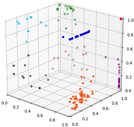
Depending on the exact parameters, we're likely to get a result that "looks like" this agent_count=200, round_count=20, question_count=3, trial_count=50, mistrust=2 run—

3D scatterplot of agents' beliefs after 20 rounds, split into color-coded clusters instead of all converging on the red "corner of Truth" point

Some of the agents (depicted in red) have successfully converged on the corner of Truth, but the others have polarized into factions that are all wrong about something. (The colors in the pretty 3D scatterplot are a k-means clustering for k := 8.) On average, evidence pushes our agents towards Truth—note the linearity of the blue and purple points, illustrating convergence on two out of the three problems—but agents who erroneously believe that A is better (due to some combination of a bad initial credence and unlucky experimental results that failed to reveal B's ε "edge" in the sample size allotted) can end up too far away to trust those who are gathering evidence for, and correctly converging on, the superiority of B.

Our authors wrap up:

[T]his result is especially notable because there is something reasonable about ignoring evidence generated by those you do not trust—particularly if you do not trust them on account of their past epistemic failures. It would be irresponsible for scientists to update on evidence produced by known quacks. And furthermore, there is something reasonable about deciding who is trustworthy by looking at their beliefs. From my point of view, someone who has regularly come to hold beliefs that diverge from mine looks like an unreliable source of information. In other words, the updating strategy used by our agents is defensible. But, when used on the community level, it seriously undermines the accuracy of beliefs.

I think the moral here is slightly off. The specific something reasonable about ignoring evidence generated by those you do not trust on account of their beliefs, is the assumption that those who have beliefs you disagree with are following a process that produces systematically misleading evidence. In this model, that assumption is just wrong. The problem isn't that the updating strategy used by our agents is individually "defensible" (what does that mean?) but produces inaccuracy "when used on the community level" (what does that mean?); the problem is that you get the wrong answer if your degree of trust doesn't match agents' actual trustworthiness. Still, it's enlighteningly disturbing to see specifically how the "distrust those who disagree" heuristic descends into the madness of factions.

(Full source code.)

Algorithms of Deception!

(originally published at Less Wrong)

I want you to imagine a world consisting of a sequence of independent and identically distributed random variables \(X_i\), and two computer programs.

The first program is called Reporter. As input, it accepts a bunch of the random variables \(X_i\). As output, it returns a list of sets whose elements belong to the domain of the \(X_i\).

The second program is called Audience. As input, it accepts the output of Reporter. As output, it returns a probability distribution.

Suppose the \(X_i\) are drawn from the following distribution:

$$P(X = x) = \begin{cases} 1/2 & x = 1 \\ 1/4 & x = 2 \\ 3/16 & x = 3 \\ 1/16 & x = 4 \\ \end{cases}$$

We can model drawing a sample from this distribution using this function in the Python programming language:

import random

def x():
    r = random.random()
    if 0 <= r < 1/2:
        return 1
    elif 1/2 <= r < 3/4:
        return 2
    elif 3/4 <= r < 15/16:
        return 3
    else:
        return 4

For compatibility, we can imagine that Reporter and Audience are also written in Python. This is just for demonstration in the blog post that I'm writing—the real Reporter and Audience (out there in the world I'm asking you to imagine) might be much more complicated programs written for some kind of alien computer the likes of which we have not yet dreamt! But I like Python, and for the moment, we can pretend.

So pretend that Audience looks like this (where the dictionary, or hashmap, that gets returned represents a probability distribution, with the keys being random-variable outcomes and the values being probabilities):

from collections import Counter

def audience(report):
    a = Counter()
    for sight in report:
        for possibility in sight:
            a[possibility] += 1/len(sight)            
    d = sum(a_j - len(a) for a_j in a.values())
    return {x: (a_i - 1)/d for x, a_i in a.items()}

Let's consider multiple possibilities for the form that Reporter could take. A particularly simple implementation of Reporter (call it reporter_0) might look like this:

def reporter_0(xs):
    output = []
    for x in xs:
        output.append({x})
    return output

The pairing of audience and reporter_0 has a Very Interesting Property! When we call our Audience on the output of this Reporter, the probability distribution that Audience returns is very similar to the distribution that our random variables are from!1

>>> audience(reporter_0([x() for _ in range(100000)]))
{1: 0.5003300528084493, 2: 0.2502900464074252, 3: 0.1873799807969275, 4: 0.062119939190270444}

# Compare to P(X) expressed as a Python dictionary—
>>> {1: 1/2, 2: 1/4, 3: 3/16, 4: 1/16}
{1: 0.5, 2: 0.25, 3: 0.1875, 4: 0.0625}

Weird, right?!

Of course, there are other possible implementations of Reporter. For example, this choice of Reporter (reporter_1) does not result in the Very Interesting Property—

def reporter_1(xs):
    output = []
    for _ in range(len(xs)):
        output.append({4})
    return output

It instead induces Audience to output a very different (and rather boring) distribution. It doesn't even matter how the \(X_i\) turned up; the result will always be the same:

>>> audience(reporter_1([x() for _ in range(100000)]))
{4: 1.0}

We could go on imagining other versions of Reporter, like this one (reporter_2)—

def reporter_2(xs):
    output = []
    for x in xs:
        if x == 4 or random.random() < 0.2:
            output.append({x})
        else:
            continue
    return output

While the distribution that reporter_2 makes Audience output isn't as boring as the one we saw for reporter_1, it still doesn't result in the Very Interesting Property of matching the distribution of the \(X_i\). It comes closer than reporter_1 did—notice how the ratios of probabilities assigned to the first three outcomes is similar to that of the original distribution—but it's assigning way too much probability-mass to the outcome "4":

>>> audience(reporter_2([x() for _ in range(100000)]))
{1: 0.3971289947471831, 2: 0.20309555314968522, 3: 0.14860259032038173, 4: 0.2516540358474678}

So far, all of the Reporters we've imagined are still only putting one element in the inner sets of the list-of-sets that they return. But we could imagine reporter_3

def reporter_3(xs):
    output = []
    for x in xs:
        if x == 1 or x == 4:
            output.append({1, 4})
        else:
            output.append({x})
    return output

Unlike reporter_2 (which typically returned a list with fewer elements than it received as input), the list returned by reporter_3 has exactly as many elements as the list it took in. Yet this Reporter still prompts Audience to return a distribution with too many "4"s—and unlike reporter_2, it doesn't even get the ratio of the other outcomes right, yielding disproportionately fewer "1"s compared to "2"s and "3"s than the original distribution—

>>> audience(reporter_3([x() for _ in range(100000)]))
{1: 0.2808949431909106, 2: 0.24795967354776766, 3: 0.19037045927348376, 4: 0.2808949431909106}

Again, I've presented Audience and various possible Reporters as simple Python programs for illustration and simplicity, but the same input-output relationships could be embodied as part of a more complicated system—perhaps an entire conscious mind which could talk.

So now imagine our Audience as a person with her own hopes and fears and ambitions ... ambitions whose ultimate fulfillment will require dedication, bravery—and meticulously careful planning based on an accurate estimate of \(P(X)\), with almost no room for error.

So, too, imagine each of our possible Reporters as a person: loyal, responsible—and, entirely coincidentally, the supplier of a good that Audience's careful plans call for in proportion to the value of \(P(X = 4)\).

When the expected frequency of "4"s fails to appear, Audience's lifework is in ruins. All of her training, all of her carefully calibrated plans, all the interminable hours of hard labor, were for nothing. She confronts Reporter in a furor of rage and grief.

"You lied," she says through tears of betrayal, "I trusted you and you lied to me!"

The Reporter whose behavior corresponds to reporter_2 replies, "How dare you accuse me of lying?! Sure, I'm not a perfect program free from all bias, but everything I said was true—every outcome I reported corresponded to one of the \(X_i\). You can't call that misleading!"

He is perfectly sincere. Nothing in his consciousness reflects intent to deceive Audience, any more than an eight-line Python program could be said to have such "intent." (Does a for loop "intend" anything? Does a conditional "care"? Of course not!)

The Reporter whose behavior corresponds to reporter_3 replies, "Lying?! I told you the truth, the whole truth, and nothing but the truth: everything I saw, I reported. When I said an outcome was a oneorfour, it actually was a oneorfour. Perhaps you have a different category system, such that what I think of as a 'oneorfour', appears to you to be any of several completely different outcomes, which you think my 'oneorfour' concept is conflating. If those outcomes had wildly different probabilities, if one was much more common than fou—I mean, than the other—then you'd have no way of knowing that from my report. But using language in a way you dislike, is not lying. I can define a word any way I want!"

He, too, is perfectly sincere.

Commentary

Much has been written on this website about reducing mental notions of "truth", "evidence", &c. to the nonmental. One need not grapple with tendentious mysteries of "mind" or "consciousness", when so much more can be accomplished by considering systematic cause-and-effect processes that result in the states of one physical system becoming correlated with the states of another—a "map" that reflects a "territory."

The same methodology that was essential for studying truthseeking, is equally essential for studying the propagation of falsehood. If true "beliefs" are models that make accurate predictions, then deception would presumably be communication that systematically results in less accurate predictions (by a listener applying the same inference algorithms that would result in more accurate predictions when applied to direct observations or "honest" reports).

In a peaceful world where most falsehood was due to random mistakes, there would be little to be gained by studying processes that systematically create erroneous maps. In a world of conflict, where there are forces trying to slash your tires, one would do well do study these—algorithms of deception!


  1. But only "very" similar: the code for audience is not the mathematically correct thing to do in this situation; it's just an approximation that ought to be good enough for the point I'm trying to make in this blog post, for which I'm trying to keep the code simple. (Specifically, the last two lines of audience are based on the mode of the Dirichlet distribution, but, firstly, that part about increasing the hyperparameters fractionally when you're uncertain about what was observed (a[possibility] += 1/len(sight)) is pretty dodgy, and secondly, if you were actually going to try to predict an outcome drawn from a categorical distribution like \(P(X)\) using the Dirichlet distribution as a conjugate prior, you'd need to integrate over the Dirichlet hyperparameters; you shouldn't just pretend that the mode/peak represents the true parameters of the categorical distribution—but as I said, we are just pretending.) 

Subzero

Python has this elegant destructuring-assignment iterable-unpacking syntax that every serious Pythonista and her dog tends to use whereëver possible. So where a novice might write

split_address = address.split(':')
host = split_address[0]
port = split_address[1]

a serious Pythonista (and her dog) would instead say

host, port = address.split(':')

which is clearly superior on grounds of succinctness and beauty; we don't want our vision to be cluttered with this ugly sub-zero, sub-one notation when we can just declare a sequence of names.

Consider, however, the somewhat-uncommon case where we have an iterable that, for whatever reason, we happen to know contains only one element, and we want to assign that one element to a variable. Here, I've seen people who ought to know better fall back to indexing:

if len(jobs) == 1:
   job = jobs[0]

But there's no reason to violate the æsthetic principle of "use a length-n (or smaller) tuple of identifiers on the left side of a destructuring assignment in order to name the elements of a length-n iterable" just because n happens to be one:

if len(jobs) == 1:
   job, = jobs

Attentional Shunt

#!/usr/bin/env python3

# Copyright © 2015 Zack M. Davis

# Permission is hereby granted, free of charge, to any person obtaining a copy
# of this software and associated documentation files (the "Software"), to deal
# in the Software without restriction, including without limitation the rights
# to use, copy, modify, merge, publish, distribute, sublicense, and/or sell
# copies of the Software, and to permit persons to whom the Software is
# furnished to do so, subject to the following conditions:

# The above copyright notice and this permission notice shall be included in
# all copies or substantial portions of the Software.

# THE SOFTWARE IS PROVIDED "AS IS", WITHOUT WARRANTY OF ANY KIND, EXPRESS OR
# IMPLIED, INCLUDING BUT NOT LIMITED TO THE WARRANTIES OF MERCHANTABILITY,
# FITNESS FOR A PARTICULAR PURPOSE AND NONINFRINGEMENT. IN NO EVENT SHALL THE
# AUTHORS OR COPYRIGHT HOLDERS BE LIABLE FOR ANY CLAIM, DAMAGES OR OTHER
# LIABILITY, WHETHER IN AN ACTION OF CONTRACT, TORT OR OTHERWISE, ARISING FROM,
# OUT OF OR IN CONNECTION WITH THE SOFTWARE OR THE USE OR OTHER DEALINGS IN
# THE SOFTWARE.

"""
Configure the machine to shunt traffic to distracting sites to localhost,
preserving attention.
"""

import os
import argparse
import subprocess
import sys
from datetime import datetime, timedelta

ETC_HOSTS = os.path.join(os.sep, 'etc', 'hosts')
HEADER = "# below managed by attentional shunt"
INVERSE_COMMANDS = {'enable': "disable", 'disable': "enable"}

DISTRACTING_HOSTS = (  # modify as needed
    'news.ycombinator.com',
    'math.stackexchange.com',
    'scifi.stackexchange.com',
    'worldbuilding.stackexchange.com',
    'workplace.stackexchange.com',
    'academia.stackexchange.com',
    'codereview.stackexchange.com',
    'puzzling.stackexchange.com',
    'slatestarcodex.com',
    'twitter.com',
    'www.facebook.com',
    'slatestarscratchpad.tumblr.com',
)
SHUNTING_LINES = "\n{}\n{}\n".format(
    HEADER,
    '\n'.join("127.0.0.1 {}".format(domain)
              for domain in DISTRACTING_HOSTS)
)


def conditionally_reexec_with_sudo():
    if os.geteuid() != 0:
        os.execvp("sudo", ["sudo"] + sys.argv)


def enable_shunt():
    if is_enabled():
        return  # nothing to do
    with open(ETC_HOSTS, 'a') as etc_hosts:
        etc_hosts.write(SHUNTING_LINES)


def disable_shunt():
    with open(ETC_HOSTS) as etc_hosts:
        content = etc_hosts.read()
    if SHUNTING_LINES not in content:
        return  # nothing to do
    with open(ETC_HOSTS, 'w') as etc_hosts:
        etc_hosts.write(content.replace(SHUNTING_LINES, ''))


def is_enabled():
    with open(ETC_HOSTS) as etc_hosts:
        content = etc_hosts.read()
    return HEADER in content


def status():
    state = "enabled" if is_enabled() else "disabled"
    print("attentional shunt is {}".format(state))


def schedule(command, when):  # requires `at` job-scheduling utility
    timestamp = when.strftime("%H:%M %Y-%m-%d")
    at_command = ['at', timestamp]
    at = subprocess.Popen(
        at_command,
        stdin=subprocess.PIPE, stdout=subprocess.PIPE, stderr=subprocess.PIPE
    )
    at.communicate(command.encode())


if __name__ == "__main__":
    arg_parser = argparse.ArgumentParser(description=__doc__)
    arg_parser.add_argument('command',
                            choices=("enable", "disable", "status"))
    arg_parser.add_argument('duration', nargs='?', type=int,
                            help=("revert state change after this many "
                                  "minutes"))
    args = arg_parser.parse_args()
    if args.command == "status":
        status()
    else:
        conditionally_reexec_with_sudo()
        if args.command == "enable":
            enable_shunt()
        elif args.command == "disable":
            disable_shunt()

        if args.duration:
            now = datetime.now()
            inverse_command = INVERSE_COMMANDS[args.command]
            schedule(
                "{} {}".format(os.path.realpath(__file__), inverse_command),
                now + timedelta(minutes=args.duration)
            )

Monthly Favorites, September 2015

Favorite commit message fragment: "it turns out that it's \d that matches a digit, whereas, counterintuitively, d matches the letter 'd'."

Favorite line of code: a tie, between

    let mut time_radios: Vec<(Commit, mpsc::Receiver<(Option<Commit>, f32)>)> =
        Vec::new();

and

        for (previous, new), expected in zip(
                itertools.product(('foo', None), ('bar', None)),
                ("from foo to bar", "from foo", "to bar", "")):

(Though both of these contain at least one internal newline, it's only for PEP 8-like reasons; they're both what we would intuitively call one "logical" line of code.)

Favorite film: My Little Pony: Equestria Girls: Friendship Games. (Poor plotting even by Equestria Girls standards, and it could only have been because of magic that I didn't get semantically satiated on the word magic during the climax. Alternate-Twilight's idiotic decision to withdraw her application to the Everton independent study program in favor of transferring to the Canterlot School of Mediocrity and Friendship in order to be closer to the Humane 5+1 was as predictable as it was disappointing—though I do credit the writers for at least acknowledging the existence of alternatives to school. And what was up with that scene where we're momentarily led to believe that alternate-Spike got switched up with Equestria-Spike in a portal accident, but then it turns out that, no, alternate-Spike just magically learned how to talk? Is it that there was no time in the script to deal with the consequences of swapping sidekicks across worlds, but that Cathy Weseluck's contract guaranteed her a speaking role? Despite being the weakest film in the trilogy (far worse than its brilliant predecessor, My Little Pony: Equestria Girls: Rainbow Rocks), Friendship Games is still a fun watch, and an easy favorite during a month when I didn't see any other feature-length films.)

RustCamp Reminiscences

On Saturday the first, I attended RustCamp, the first conference dedicated to the newish (in development for fiveish years, but having just hit version 1.0.0 this May, with all the stability guarantees that implies under the benevolent iron fist of semantic versioning) programming language Rust!

a RustCamp conference badge on a lanyard, resting on a black t-shirt printed with a gold dragon design and the text "Enter the Monad"

Why RustCamp? (It's a reasonable rhetorical question with which to begin this paragraph: going to a conference has opportunity costs in time and money; things worth blogging about are occasionally worth justifying—even if no one actually asked me for a justification.) A lot of the answer can be derived from the answer to a more fundamental question, "Why Rust?" And for me, I think a lot of the answer to that has to do with being sick of being a fake programmer living in a fake world that calls itself Python.

Don't get me wrong: Python is a very nice place to live: good weather, booming labor market, located in a good school district, with most of the books you might want already on the shelves of the main library and almost all of the others a mere hold request away. It's idyllic. Almost ... too idyllic, as if the trees and swimming pools and list comprehensions and strip malls are conspiring to hide something from us, to keep us from guessing what lurks in the underworld between the lines, the gears and gremlins feeding and turning in the layers of tools built on tools built on tools that undergird our experience. True, sometimes small imperfections in the underworld manifest themselves as strange happenings that we can't explain. But mostly, we don't worry ourselves about it. Life is simple in Python. We reassure our children that that legends of demon-king Malloc are just stories. Everything is a duck; ducks can have names and can be mutable or immutable. It all just works like you would expect from common sense, at least if you grew up around here.

And it's all fake. A child's world of rounded edges and plastic safety guards. The laws of nature wouldn't permit it to exist on its own. The old legends are true; you can't just create objects without space to put them in. But space has to be allocated, managed. Those who are brave and wise enough to study the ancient lore know how even our simplest thoughts, like setting a key in a dictionary or __init__alizing an instance of a class, are really implemented in some sort of nest of pointers traversing pointers in the underworld. I don't want to stay in my hometown forever; I want to follow the heroine's path and probe the true secrets of the underworld, to wield the virtues of our ancestors and summon the strength to lift worlds. But my wording is deliberate: the virtues of the ancestors, but not necessarily their tools. Even the greatest among us are prone to mistype or misthink; the legends tell us of lives and worlds destroyed by buffers overrun, or by trying to occupy space after the counterspell to disperse it has been cast. Lately, I had been hearing rumors of a new lore, one that grants access to the underworld and its unfathomable performance, while maintaining protective wards to shield casters from most of the inherent dangers. I had already experimented with it for a few toy programs (and used it as a bad compiler target); I made pilgrimage to the camp to learn more.

Or at least, to be inspired to more. That's most of my answer to the rest of the "Why RustCamp?" question. I'm skeptical that anyone actually learns much at conferences (lectures are notoriously less efficient than text, and mere reading needs to be combined with many, many hours of hacking to produce true skill), but getting together with people, attentively listening to them yap on stage, and mingling with the crowd during breaks, provides pointers to things to read and hack on later in addition to serving certain human social needs, giving one the strength to carry on trying to better one's mastery of one's chosen profession, even through the persistent suspicion that it none of it helps, that the young programmer's vaunted "passion" is all vanity and empty signaling that will soon be destroyed by the realization that your code doesn't really change users' lives in any appreciable way, and no one cares how smart you are. (Enjoy Arby's.)

I felt lucky that the event happened to be on my side of the bay, in Berkeley, given that the trains to the city were 503ing this weekend on account of scheduled downtime for essential security patches. On the walk from Downtown Berkeley station, I stopped at one of the outposts of the rival power to buy a specialty medicinal and a scone. I usually go to the American coffee hegemon, but the rival power has this this newish specialty medicinal, an iced-coffee with one-and-a-half kinds each of cream and sweetener, that, having tried it for the first time the day before, I privately think beats anything in the hegemon's arsenal.

I made my way to the event venue and checked in, receiving a pretty badge and the obligatory swag bag containing an event-logo tee, a tee with a clever functional-programming-dragon design on the front and a sponsor logo on the back, bottled water (which is ridiculous), a Wi-Fi password (I hadn't bought my laptop), and stickers (I almost never use stickers). I am illustrating this post with a photo of the badge and dragon tee because I forgot to bring a camera to take pictures at the conference itself, and—lest the reader object that only die-hard photography fanatics have dedicated cameras nowadays—I don't have a real phone. (I'm into technology, just not necessarily consumer technology. Maybe I'll upgrade when the Ubuntu phone goes on sale in the U.S., but likely not even then.)

I was mildly surprised at the number of familiar-to-me faces in attendance (from my native subculture, or indeed more specifically from the party on Thursday, or from non-Rust programming scenes), but I guess this shouldn't be surprising on anthropic grounds. I speculated that there would be a lot of relative newbies (like me) at this event as contrasted to a conference for a more established technology—more people come to RustCamp because they want to check out the hot up-and-coming new language than because they've been doing it at their dayjob for five years. (During post-registration mingling, someone mentioned wanting something like Haskell's Maybe types, and I said, "I think we call it Option around here.")

The talks were in a big room with a bunch of circular tables (the tables were also mildly surprising to me; I guess I had been expecting rows of chairs, but no doubt it's better for laptops to not literally have to rest atop laps).

First, Aaron Turon and Niko Matsakis gave a keynote (PDF) about how far Rust has come and what remains to be done on the timescale of a year or so. They mentioned that there's a tool called Crater that tests a build of the Rust compiler against the packages on crates.io, to detect regressions with respect to how people are actually writing Rust in the wild. And the 1.0.0 API stability guarantee certainly doesn't mean there's not a lot of work left to do on the compiler. Apparently, as of now, rustc builds a big AST of your entire crate and hands that off to LLVM, which can lead to disappointingly slow compile times for large crates, but people are working on a more modular "middle intermediate representation" that will allow fast, incremental compilation at the level of individual functions. There's also work on making the borrow checker less dumb (in the matter of rejecting perfectly good code that it doesn't yet know how to prove is safe), and IDE support ("It's come to my attention that some people are not satisfied with Emacs"). In the gap after the keynote but before the first non-keynote presentation, I had a good conversation about cartoons with a fellow attendee.

Alexis Beingessner gave a really informative talk that the program called "Who Owns This Stream of Data?", but which the slides called "OMG ITERATORS". Beingessner's presentation style seems to be characterized by a kind of affectedly enthusiastic Buffy Speak that I can't quite bring myself to criticize, but only because I expect people would say similar (though not identical) things about my writing. In the toy Rust programs I've written so far, I've gotten used to calling .iter() on a vector in order to iterate over it in a for loop. This is a part of Rust's Iterator trait, implementations of which have to provide a next function that returns an Option of the type you're iterating over. (It's just like Python, except that in Python the method names have double underscores around them, for implicitly calls .__iter__() for you, and we raise StopIteration instead of returning the None alternative of an Option!) But it turns out that Rust actually had other kinds of iterators that correspond to different ways of using Rust's ownership system (where multiple things can have a read-only reference to a piece of data, but only one thing can have the ability to write to it at a time in accordance with "ownership" and "borrowing" rules that I don't really understand yet). So .iter() gives shareable immutable references, .iter_mut() gives restricted-use mutable references, and .into_iter() actually moves the data out of the collection (almost like a Python generator, which can't be reset once exhausted). And there was something about this cool trick where you iterate over indices of a vector backwards so that you can conditionally use swap_remove to take stuff out of the middle in constant time.

Matt Cox gave a talk on "Learning Systems Programming With Rust" that I had really been looking forward to. He explained memory on the stack and the heap with cute animations of unofficial Rust mascot Ferris the crab gliding around putting values into boxes. Unfortunately, there seemed to some kind of mistake where he had an outdated version of his slides?—the talk got wrapped up awkwardly, and I wish we had gotten to hear the rest of what he had in mind.

There were a few talks about some companies' experience actually using Rust in production, and somebody wrote a clone of Graphite in Rust. Somehow I don't have a whole lot to say about these.

I really liked Carol (Nichols || Goulding)'s presentation on doing code archaeology with Git, issue trackers, and mailing list archives. The topic was dear to my heart, given how much of a Git-blame–intensive workflow I have (I M-x vc-annotate constantly). During the second example, on using blame and log to track down the origin of the lifetime elision rules, I found myself wondering if she was going to mention the Git log pickaxe and whether I should try to bring it up in Q&A if she didn't. Then she did discuss it in the third example, mentioning in passing that she didn't know why it was called the pickaxe. Someone in the audience tried to argue that the -S switch resembled a pickaxe. "No, it does not look like a pickaxe," (Nichols || Goulding) replied, "I don't think you could cut down any trees with a dash capital-S."

Carl Lerche talked about his Mio library for asynchronous I/O in Rust; I also don't have a much to say about that one, except that the typography on his slides was very tastefully done.

Yehuda Katz (of Bundler and jQuery fame, amongst others) talked about how to call Rust code from C (or your favorite other language via C extensions). "Rust," he argued, "is a DSL for describing ownership concepts that you have to think about while using C or C++." He recommended that for anything more complicated than simple numerical types, you should translate Rust types to an opaque void * pointer in your C code, and put that in your language's object type if you're writing a C extension. (You can write and expose Rust functions to do useful things with it.)

Finally, Nick Cameron talked about using functionality of the compiler to write tools for Rust, like extra linters and smart code search. Listening to him actually gave me a cool project idea that has nothing to do with Rust, namely that you could write a tool using Python's ast module to count how often which variable names are used, and cross-reference it with Git blame (the AST-node objects know what line number they're from) to see if different members of your team make noticeably different variable name choices.

So that was RustCamp! It was fun, but if I want the fun to have meant anything in the end, I'll have to put more effort into learning Rust properly.

$

I used to think of $ in regular expressions as matching the end of the string. I was wrong! It actually might do something more subtle than that, depending on what regex engine you're using. In my native Python's re module, $

[m]atches the end of the string or just before the newline at the end of the string, and in MULTILINE mode also matches before a newline.

Note! The end of the string, or just before the newline at the end of the string.

In [2]: my_regex = re.compile("foo$")

In [3]: my_regex.match("foo")
Out[3]: <_sre.SRE_Match object; span=(0, 3), match='foo'>

In [4]: my_regex.match("foo\n")
Out[4]: <_sre.SRE_Match object; span=(0, 3), match='foo'>

I guess I can see the motivation—we often want to use the newline character as a terminator of lines (by definition) or files (by sacred tradition), without wanting to think of \n as really part of the content of interest—but the disjunctive behavior of $ can be a source of treacherous bugs in the fingers of misinformed programmers!

It happened to me while I was doing speculative pre-development of the speculative pre-prototype for my speculative Glitteral programming language, specifically in the lexical analyzer—the part of a compiler that recognizes strings of source code as representing tokens that mean something in the language's grammar: this is a language keyword, that's an integer literal, this is an identifier, and so forth. My makeshift lexical analyzer (inspired by, but diverging significantly from, the more sophisticated thing that textbook said to do—I was in a hurry) involved deciding if a segment of source code could represent a particular token (or prefix thereof) by checking if it matched the regular expression defining each token class (or a regex describing prefixes of that token class). I had prudently (but not prudently enough, as you see) anchored each of my token class regexes with $, so that, for example, the source fragment fore could not be erroneously recognized as the language keyword for. But that just left me with a bug in which a newline immediately following a token would be recognized as part of the token: for example, you could end up lexing the string 3\n as an integer literal, even though the integer literal was supposed to be just 3. After my first crude fix later proved to be inadequate, I ended up fixing it by augmenting the $s with the negative lookahead assertion (?!\n) immediately thereafter, in effect saying, "match the end of the string or just before the newline at the end of the string, but not just before a newline," the negative lookahead assertion canceling out the interpretation of $ that I didn't want. And then later I replaced all those $(?!\n)s with \Zs (which actually match the end of the string, like I wanted in the first place), after it was brought to my attention that \Z was a thing.

But I'm not the only one who was confused! (Note: the previous sentence should be read in a tone of terror and despair at the tightness of the cruel grip of ignorance on our fragile world, not relief that other people are as dumb as me.) The famous Django web application framework recently released patch versions 1.8.3, 1.7.9, and 1.4.21 due to security concerns, one of which being validators failing to guard against possible header injection vulnerabilities owing to the use of $ instead of \Z in regular expressions.

All this that I have said about $ in regexes concerns the Python world. Apparently Perl is the same way (maybe we got it from them?). But other regex engines don't have the "or just before the newline" semantic flourish in their interpretation of $. In Java, for example (and therefore, more importantly from my point of view, Clojure),

[b]y default, the regular expressions ^ and $ ignore line terminators and only match at the beginning and the end, respectively, of the entire input sequence.

user=> (re-matches #"foo$" "foo")
"foo"
user=> (re-matches #"foo$" "foo\n")
nil

Whereas in Ruby, $ is explicitly the end of line anchor (like in Python's MULTILINE mode), \Z matches the end of the string or just before the newline if the string ends with a newline (like Python's default), and \z is for the end of the string!

I guess the moral is that if you want to write a kind of regular expression that you're not already intimately familiar with, you should think carefully and read the owner's manual of your chosen regex engine. What you find there may surprise you!

__pycache__/shibboleth.cpython-34.pyc

Sometimes I worry that people with power in Society will look down on me for my pronunciation of the .pyc extension for Python bytecode files. I always want to say pike-cee, even though many would argue that the c should either be hard (pike) or said as the name of the letter (py-cee), but certainly not both in sequence!

The Foundations of Erasure Codes

(cross-posted from the SwiftStack Blog)

In enabling mechanism to combine together general symbols, in successions of unlimited variety and extent, a uniting link is established between the operations of matter and the abstract mental processes of the most abstract branch of mathematical science. A new, a vast, and a powerful language is developed for the future use of analysis, in which to wield its truths so that these may become of more speedy and accurate practical application for the purposes of mankind [sic] than the means hitherto in our possession have rendered possible.

Ada Lovelace on Charles Babbage's Analytical Engine, 1842

Dear reader, if you're reading [the SwiftStack Blog], you may have already heard that erasure codes have been added to OpenStack Swift (in beta for the 2.3.0 Kilo release, with continuing improvements thereafter) and that this is a really great thing that will make the world a better place.

All of this is entirely true. But what is perhaps less widely heard is exactly what erasure codes are and exactly why their arrival in Swift is a really great thing that will make the world a better place. That is what I aim to show you in this post—and I do mean show, not merely tell, for while integrating erasure codes into a production-grade storage system is (was!) an immense effort requiring months of work by some of the finest programmers the human race has to offer, the core idea is actually simple enough to fit in a (longish) blog post. Indeed, by the end of this post, we will have written a complete working implementation of a simple variant of Reed–Solomon coding, not entirely unlike what is used in Swift itself. No prior knowledge will be assumed except a working knowledge of high-school algebra and the Python programming language.

But first, we need to understand the problem that erasure codes solve. The strategy Swift has traditionally used to achieve its reliability and fault-tolerance properties is replication: keep more than one copy of each object (typically three), preferably in entirely different datacenters, failing that, on different machines, and failing that, at least on different hard drives. Your data is safe from occasional drive failures because the probability of all the drives containing a particular object failing at the same time is very, very small.

The problem with replication is that it's expensive: if you keep three replicas, then for every terabyte that you want to use, you have to pay for three terabytes of actual physical storage. The cost would appear to be unavoidable, unless ... unless there were some way to reap the benefits of distributing the information across different failure domains without storing the entire object at each location ...

"But surely this is impossible!" I hear you cry. "It's useless to make half a copy of something, because you can't know in advance of a disaster whether the half you made a backup of is the half that will need to be restored. In order to enjoy the safety of having a spare, you need a spare of the whole thing."

My dear reader, this objection is compelling, well-stated—and gloriously, one-hundred-percent wrong. We can achieve reliability guarantees similar to that of the replication strategy, keeping our data safe even as some of its fragments are damaged, lost, or erased. (Hence the name, erasure codes.) The method will have its own costs in the form of increased CPU load and more network requests; it won't make sense for all use cases, but when appropriate, the efficiency gain is impressive. It all depends on applying a deep philosophical insight into the nature of space itself.

Specifically: two points make a line.

Given any two distinct points on a plane, there is one and exactly one line that passes through both of them. We reconstruct anything we might want to know about a particular line just by remembering two points that it passes through.

But suppose we were to remember three points. Then we could still reconstruct the line from any two of them, which means that the information about our line hasn't been lost even if we forget one of the points.

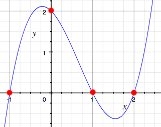
graph of a cubic polynomial curve passing through four marked points

Similarly, three points make a parabola, four points make a cubic curve, and in full generality, m+1 points make a degree-m polynomial. Given n points on a polynomial curve where n is greater than m+1, any m+1 of them suffice to reconstruct the polynomial.

Thus, we have a clear strategy for storing data in a reliable, failure-tolerant way, without going to the expense of storing complete replicas: all we have to do is pretend our data is made out of polynomials, and store more points than are strictly necessary to reconstruct the data.

But don't take my word for it! Mere verbal arguments can be deceptive, but code is proof and code is truth, so if you still doubt that such an idea can really be made to work—and maybe you should—you won't after we're done implementing it.

So suppose we want to save some textual data; say, the string, "THE FUNDAMENTAL PROBLEM OF COMMUNICATION IS THAT OF REPRODUCING AT ONE POINT EITHER EXACTLY OR APPROXIMATELY A MESSAGE SELECTED AT ANOTHER POINT". Now, this data is made out of letters and spaces, not polynomials, but we can process it into a form that will make it easier to make-believe that it is. Say, we split the text into chunks of a fixed size (padding the end with extra spaces if necessary so that our chunk size evenly divides it), and convert the characters into integers from 0 to 26 (space is 0, A is 1, B is 2, &c.). Here are some functions to help with that—

from string import ascii_uppercase

ALPHABET = " "+ascii_uppercase
CHAR_TO_INT = dict(zip(ALPHABET, range(27)))
INT_TO_CHAR = dict(zip(range(27), ALPHABET))

def pad(text, chunk_size):
    return text + ' '*(chunk_size - len(text) % chunk_size)

def chunkify(text, chunk_size):
    return [text[i:i+chunk_size]
            for i in range(0, len(text), chunk_size)]

def convert(string):
    return [CHAR_TO_INT[c] for c in string]

After turning our text into converted chunks (lists of integers), we can interpret each chunk as representing the coefficients of a polynomial function: say, in order of increasing degree, so that, e.g., the list [1, 2, 3] represents the function \(1 + 2x + 3x^2\). Then we can take points on that polynomial at \(n\) different values of the independent variable \(x\) for some \(n\) greater than the chunk size to get a properly redundant encoding.

(It's actually better if you use polynomials over the finite field \(\mathbb{F}_q\) of the integers modulo \(q\) for some \(q\) which is a prime raised to the power of something, but let's not worry about that.)

def evaluate_polynomial(coefficients, x):
    return sum(c * x**i for i, c in enumerate(coefficients))

def encode(chunk, n):
    return [evaluate_polynomial(chunk, i) for i in range(n)]

def erasure_code(text, chunk_size, encoded_chunk_size):
    chunks = chunkify(pad(text, chunk_size), chunk_size)
    converted_chunks = [convert(chunk) for chunk in chunks]
    return [list(enumerate(encode(chunk, encoded_chunk_size)))
            for chunk in converted_chunks]

Then, with a choice for the original chunk size (which you'll recall will also be the number of terms each in the polynomials used to encode each chunk) and the size of the resulting encoded chunk (that is, the number of points we'll sample from the polynomials), we can encode our text.

$ python3
>>> from reed_solomon import *
>>> text = "THE FUNDAMENTAL PROBLEM OF COMMUNICATION IS THAT OF
REPRODUCING AT ONE POINT EITHER EXACTLY OR APPROXIMATELY A MESSAGE
SELECTED AT ANOTHER POINT"
>>> encoded = erasure_code(text, 5, 8)
>>> encoded
[[(0, 20), (1, 39), (2, 152), (3, 575), (4, 1668), (5, 3935), (6,
8024), (7, 14727)], [(0, 21), (1, 53), (2, 281), (3, 1179), (4, 3533),
(5, 8441), (6, 17313), (7, 31871)], [(0, 5), ...

[further output redacted]

At this point, our text has been transformed into a Python list, whose elements are Python lists representing the individual chunks, whose elements are tuples representing (x, y) coordinate pairs representing points on the polynomial representing that chunk.

Let's simulate distributing that encoded information across several storage nodes by writing points with different x-values to different files. We'll make-believe that each file is a different storage node. We'll write another function for that.

import json

def disperse(encoded_chunks):
    node_count = len(encoded_chunks[0])
    for i in range(node_count):
        with open('node'+str(i), 'w') as node:
            node.write(json.dumps([chunk[i] for chunk in encoded_chunks]))

And try it out—

>>> disperse(encoded)
>>>
$ ls
node0  node1  node2  node3  node4  node5  node6  node7
$ cat node4
[[4, 1668], [4, 3533], [4, 3517], [4, 1824], [4, 4080], [4, 4342],
[4, 1665], [4, 4769], [4, 5460], [4, 4172], [4, 4710], [4, 2254], [
4, 433], [4, 2436], [4, 4464], [4, 5796], [4, 1596], [4, 4428], [4,
 1417], [4, 5313], [4, 5452], [4, 709], [4, 6212], [4, 4973], [4, 5
445], [4, 5205], [4, 6308], [4, 4412], [4, 1555]]

In conclusion, that's how you use Reed–Solomon coding to turn comprehensible English text into inscrutable lists of lists of numbers distributed across several files. Thank you, and—

What's that you say, dear reader? Demonstrating how to encode something is useless unless you also demonstrate how to decode it? Well, I suppose you may have a point. Never fear—we can do that, too! But first, we'll need some functions for manipulating polynomials (in the "list of coefficients in order of ascending power" form that we've been using).

def get_coefficient(P, i):
    if 0 <= i < len(P):
        return P[i]
    else:
        return 0

def add_polynomials(P, Q):
    n = max(len(P), len(Q))
    return [get_coefficient(P, i) + get_coefficient(Q, i) for i in range(n)]

def scale_polynomial(P, a):
    return [a*c for c in P]

def multiply_polynomials(P, Q):
    maximum_terms = len(P) + len(Q)
    R = [0 for _ in range(maximum_terms)]
    for i, c in enumerate(P):
        for j, d in enumerate(Q):
            R[i+j] += c * d
    return R

Once we can do arithmetic with polynomials, we can write functions to reconstruct the polynomial representing a chunk of our text given our saved points, which is probably the most intricate part of this entire endeavor. We'll use a technical trick called Lagrange interpolation, after the great mathematician-astronomer Joseph-Louis Lagrange.

Suppose we want to reconstruct a cubic polynomial from the four points \((x_1, y_1)\), \((x_2, y_2)\), \((x_3, y_3)\), and \((x_4, y_4)\). It turns out that a formula for the polynomial is

$$y_1\ell_1(x) + y_2\ell_2(x) + y_3\ell_3(x) + y_4\ell_4(x)$$

where \(\ell_1(x)\) (the first Lagrange basis element) stands for

$$\frac{(x - x_2)(x - x_3)(x - x_4)}{(x_1 - x_2)(x_1 - x_3)(x_1 - x_4)}$$

and so on—for each \(i\) between 1 and the number of points we have, the numerator of the \(i\)th Lagrange basis element is the product of \((x - x_j)\) for all \(j\) from 1 up to the number of points we have but not equal to \(i\), and the denominator follows a similar pattern but with \(x_i\) instead of \(x\). (Note that we're using letters with subscripts, like \(x_i\), to represent specific constants, whereas \(x\) without a subscript is a function's independent variable.)

I hear you ask, "But why this particular arbitrary-looking formula out of the space of all possible arbitrary-looking formulae?" But the grace and beauty of this formula is exactly that it's engineered specifically to pass through our points. Consider what happens when we choose \(x\) equal to \(x_1\). The second through fourth terms \(y_2\ell_2(x_1)\) through \(y_4\ell_4(x_1)\) all contain a factor of \((x_1 - x_1)\) and are thus zero, but the first term becomes

$$y_1\frac{(x_1 - x_2)(x_1 - x_3)(x_1 - x_4)}{(x_1 - x_2)(x_1 - x_3)(x_1 - x_4)}$$
$$= y_1(1)$$
$$= y_1$$

So by design, our interpolated polynomial takes value \(y_1\) at \(x_1\), \(y_2\) at \(x_2\), and so forth. In Python, the whole process looks like this—

def lagrange_basis_denominator(xs, i):
    denominator = 1
    for j, x in enumerate(xs):
        if j == i:
            continue
        denominator *= xs[i] - xs[j]
    return denominator

def lagrange_basis_element(xs, i):
    element = [1]
    for j in range(len(xs)):
        if j == i:
            continue
        element = multiply_polynomials(element, [-xs[j], 1])
    scaling_factor = 1/lagrange_basis_denominator(xs, i)
    return scale_polynomial(element, scaling_factor)

def interpolate(points):
    result = [0]
    xs, ys = zip(*points)
    for i in range(len(points)):
        result = add_polynomials(
            result,
            scale_polynomial(lagrange_basis_element(xs, i), ys[i])
        )
    return [round(k) for k in result]

(Note that we're rounding off our computed coefficients because this implementation isn't very numerically stable—the subtle differences between true real-number arithmetic and the approximate floating-point arithmetic implemented by computers start to accumulate, and if we choose too large of a chunk size, our program will actually start giving the wrong answers—but let's not worry about that, either.)

With this technique, we now have all the tools we need to recover our text from a subset of the data we wrote to our various "nodes" earlier. What we need to do is this: for each chunk, arbitrarily select a number of stored points equal to our chunk size, interpolate the polynomial from them, deconvert the numbers which are the coefficients of that polynomial back into their character equivalents, unchunkify the chunks into a unified whole, and unpad any whitespace we added to the end when we began.

def deconvert(sequence):
    return ''.join(INT_TO_CHAR[i] for i in sequence)

def unchunkify(chunks):
    return ''.join(chunks)

def unpad(text):
    return text.rstrip()

def erasure_decode(encoded_chunks, chunk_size, encoded_chunk_size):
    converted_chunks = [interpolate(chunk[:chunk_size])[:chunk_size]
                        for chunk in encoded_chunks]
    return unpad(unchunkify(deconvert(chunk) for chunk in converted_chunks))

But about that data that we wrote out earlier.

$ ls
node0  node1  node2  node3  node4  node5  node6  node7

It would hardly be a compelling test of our erasure-coding skills if there were any suspicion that we actually needed all of those files—we really only need as many as our chunk size. So let's suppose that three of our nodes die in a fire—

$ rm node1 node3 node6
$ ls
node0  node2  node4  node5  node7

Could this the end of our data? With a full three-eighths of our encoding having been utterly destroyed, is it delusional to hold out hope that our text might yet be faithfully recovered? No! No, it is not! We only need one more function to retrieve the encoded chunks—

def retrieve(*nodes):
    responses = []
    for node in nodes:
        with open(node) as our_node:
            responses.append(json.loads(our_node.read()))
    return [[response[i] for response in responses]
            for i in range(len(responses[0]))]

—and then—

$ python3
>>> from reed_solomon import *
>>> node_data = retrieve("node0", "node2", "node4", "node5", "node7")

—successfully decode them!

>>> erasure_decode(node_data, 5, 8)
'THE FUNDAMENTAL PROBLEM OF COMMUNICATION IS THAT OF REPRODUCING AT
 ONE POINT EITHER EXACTLY OR APPROXIMATELY A MESSAGE SELECTED AT AN
OTHER POINT'

Dear reader, it is true our toy implementation here was crude, the hundred-and-change bytes of data we demonstrated it on was of no intrinsic interest, and many obvious and not-so-obvious subtleties were ignored. But I implore you to consider the implications for your own storage needs of more advanced, not-merely-educational application of these vast and powerful techniques. Imagine just how soundly you'll be able to sleep at night knowing that you're well under your budget and yet your data is just as safe as if you had three complete independent copies of it!

And even if you personally have no intention of deploying Swift—as my SwiftStack colleague and project technical lead for OpenStack Swift John Dickinson has pointed out, we are rapidly entering an era in which everyone uses object storage, whether they realize it or not. In a hyperconnected global economy, even minor efficiency improvements in key infrastructure components can reap enormous benefits elsewhere, which is to say that the rest of your life will contain more happiness and less pain if the financial institution that invests your retirement savings, or the medical research institute that develops a cure for the cancer you'll get twenty years from now, or the image hosting service that serves you cute cat pictures today, have access to cheaper, faster, and more reliable storage than the means hitherto in our possession have rendered possible. And that's why erasure codes being in OpenStack Swift is a really great thing that will make the world a better place; quod erat demonstrandum.

The code in this post is available separately.

Mock

Some people, when confronted with a Python unit-testing problem, think, "I know, I'll use mock." Now they have <MagicMock name='two_problems' id='140279267635776'>.

Native Tongue

"Don't you ever get tired of coding everything in Python?"

"Do you ever get tired of saying everything in English?"

A beat. In unison: "Yes."

Last Friday Night

it's a blacked-out blur, but I'm pretty sure

* * *

$ heroku create
Creating howling-nightmare-4505... done, stack is cedar
http://howling-nightmare-4505.herokuapp.com/ | git@heroku.com:howling-nightmare-4505.git
Git remote heroku added

"Did they—did they change their random words dictionary for Halloween?"

* * *

-----> Python app detected
-----> Installing runtime (python-2.7.8)

"What?! No! What are you doing, you crazy machine?!"

* * *

$ echo "python-3.4.1" > runtime.txt
$ g a .
$ gco -m "the month of July 2010 called and wants their programming language back"

* * *

< What are you spinning up the box for?

it's Friday night

< How does that lead to box spinning?

previous message was an attempt at humor, as if to suggest that I'm the sort of person for whom deploying a web application fulfills a similar purpose as some sort of wild social event with drugs might for some others, about which they might offer a similarly vacuous "explanation"

* * *

it ru-uled

My Favorite Error Message This Year

zmd@SuddenHeap:~/Code/Finetooth$ git commit --amend
Traceback (most recent call last):
  File "./manage.py", line 8, in <module>
    from django.core.management import execute_from_command_line
ImportError: No module named django.core.management

Debugging Techniques I

#def my_problematic_function(x):
def my_problematic_function(x, call_count=[]):
    call_count.append(1)
    print("ZMD DEBUG call #{}".format(len(call_count)))
    import traceback; traceback.print_stack()
    result = do_stuff(x)
    etc()

Growl

Dear reader, imagine you have an idea for a work of prose that you want to have finished by Election Day for reasons which will become clear later, and you're not sure how long it should end up being, but you think maybe around twelve thousand words. When considering what you can do to ensure that this feat will actually be accomplished, it occurs to you that you could start writing now. Or

Or you could design a script to make desktop notifications about how much more writing you have to do! (Maybe you could even put it in a cronjob so that it would nag you to write automatically!)

Well, I already made it for you (unless your Linux distribution doesn't use notify-send or you're on a Mac or something).

#!/usr/bin/env python3

import argparse
import subprocess
from datetime import datetime

arg_parser = argparse.ArgumentParser()
arg_parser.add_argument("filename", help="path to file of draft")
arg_parser.add_argument("goal", type=int, help="goal wordcount")
arg_parser.add_argument("deadline", help="deadline in YYYY-MM-DD format")
args = arg_parser.parse_args()

today = datetime.today()
filename = args.filename
goal = args.goal
deadline = datetime.strptime(args.deadline, "%Y-%m-%d")

def nag_message():
    progress = int(subprocess.check_output(["wc", filename, "-w"]).split()[0])
    to_go = goal - progress
    days_remaining = (deadline - today).days
    to_go_per_day = to_go / days_remaining
    proportion = progress / goal
    return "\n".join(
        "{}: {:.2f}".format(k.replace("_", " "), v) for k, v in locals().items()
    )

subprocess.check_output(["notify-send", "writing progress", nag_message()])

My Wordcount Notification

You're welcome. Now get back to work.

Clarity of Intent

<bob> and here on line 79---
<bob>         else:
<bob>             return None
<bob> you don't need the else
<bob> Python functions will implicitly return None
<alice> $ python -c "import this" | sed -n 4p

Huffman

Dear reader, you know what's way more fun than feeling sad about the nature of the cosmos? Data compression, that's what! Suppose you want to send a message to your friends in a nearby alternate universe, but interuniversal communication bandwidth is very expensive (different universes can't physically interact, so we and our alternate-universe analogues can only communicate by mutually inferring what the other party must be saying, which takes monstrous amounts of computing power and is not cheap), so you need to make your message as brief as possible. Note that 'brief' doesn't just have to do with how long your message is in natural language, it also has to do with how that message is represented over the transuniveral communication channel: indeed, the more efficient the encoding, the more you can afford to say on a fixed budget.

The classic ASCII encoding scheme uses seven bits to represent each character. (Seven?—you ask perplexedly, surely you mean eight? Apparently it was seven in the original version.) Can we do better? Well ... ASCII has a lot of stuff that arguably you don't need that badly. Really, upper and lower case letters? Ampersands, asterisks, backslashes? And don't get me started about those unprintable control characters! If we restrict our message to just the uncased alphabet A through Z plus space and a few punctuation marks, then we can encode our message using only a 32 (= \(2^5\)) character set, at five bits per character.

Can we do better? Seemingly not—\(2^4 = 16\) isn't a big enough character set to cover the alphabet. Unless ...

Unless we abandon the assumption that each character needs to be represented by the same number of bits!

Adopting such a variable-length character encoding scheme couldn't help us if all possible messages were equally likely, but this is manifestly not true of the sort of messages anyone would actually want to send: the letter e is more common than the letter q; the word the more common than the string zkb. We can take advantage of the regularities in the sort of messages people would actually want to send by adopting a variable-length encoding scheme that assigns shorter codes to characters that occur more frequently. But then since we can no longer rely on each n bits (for some fixed n) representing one character, we'll also want our encoding scheme to be prefix-free: no character code should be a prefix of any other. That way, our message is unambiguous: if the message starts with (say) 010, which represents (say) e, then we know that the first character is e, because there won't be any other characters with codes that start with 010 (like say 01011).

Consider the process of decoding a prefix-free code: we read bits from the start of the message until we recognize a valid character code. We can visualize this graphically in the form of a binary tree with the characters in our character set at the leaves: start at the root, and then go the the left child if the first bit is 0, and the right child if it's 1, and so on until you reach a leaf, the path taken representing the code for the character at that leaf. The task of constructing such an optimal such tree (and thereby, an optimal prefix-free code) given the relative frequencies of the characters (either in a particular message, or a general class of messages that people would actually want to send) is solved by a algorithm due to David A. Huffman, which we'll implement here in Python.

First, we'll need a data structure to represent the nodes of the tree. Actually, we'll use a structure that represents a node and all of its children, which we'll call Subtree. Each instance of Subtree will have fields for a character and frequency associated with a node, and the node's left and right children if any (which are also instances of Subtree).

class Subtree:
    def __init__(self, char, freq, left, right):
        self.char = char
        self.freq = freq
        self.left = left
        self.right = right

The leaf nodes of our tree will have the character field set to a character in our set, the frequency field set to the frequency of that character, and the left and right children fields set to None. The internal nodes of the tree will have the character field set to None and the frequency field set to the sum of the frequencies of its children.

We'll also want nodes to be comparable by their frequencies:

    def __gt__(self, othernode):
        return self.freq > othernode.freq

When all is said and done, Huffman's algorithm will give us an instance of Subtree representing our tree, but it would really be more convenient to have the decoding information embodied by the tree in the form of Python dictionary mapping bitstrings to the characters they encode. We can get this by doing a standard recursive tree walk:

    def codebook(self):
        codes = {}
        def traversal(item, code):
            if item != None:
                traversal(item.left, code+'0')
                if item.char != None:
                    codes[item.char] = code
                traversal(item.right, code+'1')
        traversal(self, '')
        return codes

We're also going to need a min-priority queue, a dynamic set from which we can insert items and retrieve the "smallest":

class MinPriorityQueue:
    def __init__(self):
        self.queue = []

    def put(self, item):
        self.queue.append(item)
        self.queue.sort(reverse=True)

    def get(self):
        return self.queue.pop()

Now that we have the appropriate data structures, we're ready for Huffman's algorithm. Suppose our character/frequency data are given to us in a Python dictionary C. For each character, we create an instance of Subtree to be the corresponding leaf node in our tree, and put them all in a min-priority queue. Then we build our tree from the bottom up by selecting the two lowest-frequency nodes in the queue, making them the children of a new node whose frequency is the sum of their frequencies, putting the new node back in the priority queue, and again until we've built the entire tree:

def Huffman(C):
    Q = MinPriorityQueue()
    leaves = {Subtree(k, C[k], None, None) for k in C}
    for leaf in leaves:
        Q.put(leaf)
    for i in range(len(C)-1):
        left = Q.get()
        right = Q.get()
        new_node = Subtree(None, left.freq + right.freq, left, right)
        Q.put(new_node)
    return Q.get().codebook()

And that's Huffman's algorithm. Of course, we'll also want functions for encoding and decoding a message:

def code(plaintext, codebook):
    return ''.join(codebook[c] for c in plaintext)

def decode(ciphertext, codebook):
    decodebook = {v:k for k, v in codebook.items()}
    codeword = ''
    plaintext = ''
    for i in range(len(ciphertext)):
        codeword += ciphertext[i]
        if codeword in decodebook:
            plaintext += decodebook[codeword]
            codeword = ''
    return plaintext

So, suppose you want to send your friends in a nearby alternate universe the eighty-two character message, "I USED TO WONDER WHAT FRIENDSHIP COULD BE, UNTIL YOU ALL SHARED ITS MAGIC WITH ME." If you used seven-bit ASCII, you'd have to pay the cost of transmitting 82*7 = 574 bits. But if you use a Huffman code informed by knowledge of English letter frequencies ...

eng_freqs = {'A' : 8167, 'B' : 1492, 'C' : 2782, 'D' : 4253, 'E' : 12702,
'F' : 2228, 'G' : 2015, 'H' : 6094, 'I' : 6966, 'J' : 153, 'K' : 772,
'L' : 4025, 'M' : 2406, 'N' : 6749, 'O' : 7507, 'P' : 1929, 'Q' : 95,
 'R' : 5987, 'S' : 6327, 'T' : 9056, 'U' : 2758, 'V' : 978, 'W': 2360,
'X' : 150, 'Y' : 1974, 'Z' : 74, ' ' : 13000, '.': 4250, ',': 4250}
eng_codebook = Huffman(eng_freqs)
plain = "I USED TO WONDER WHAT FRIENDSHIP COULD BE, UNTIL YOU ALL SHARED ITS MAGIC WITH ME."
cipher = code(plain, eng_codebook)

You can send this instead:

0111010111100000100111001010110110010101110101001011011001001111110101110100
0001010110101011100111111011100101101100100010000011110000101011110110011111
0010110110010101000000011100001011110001101101011110110010100010100111110001
0101010110101100100001000010101111100111001010011111010001010111011101010001
1011111110101011101001111101000001011101100110111

—which is only 353 bits, for a savings of 38.5%.

Bibliography Cormen et al., Introduction to Algorithms, third ed'n, §16.3

Computing the Arithmetic Derivative

Jurij Kovič's paper "The Arithmetic Derivative and Antiderivative" contains a curious remark in Section 1.2. Having just stated the definition of the logarithmic arithmetic derivative (\(L(n) = n'/n = \sum_j a_j/p_j\) where the prime mark indicates the arithmetic derivative, and \(\prod_i p_i^{a_i}\) is the prime factorization of \(n\)), Kovič writes:

The logarithmic derivative is an additive function L(xy) = L(x) + L(y) for any x, y ∈ ℚ. Consequently, using a table of values L(p) = 1/p (computed to sufficient decimal places!) and the formula D(x) = L(xx, it is easy to find D(n) for n ∈ ℕ having all its prime factors in the table.

... a table of values? Did I read that correctly? Surely there must be some mistake; surely a paper published in 2012 can't expect us to rely on a printed table, for all the world as if we were John Napier in the seventeenth century! But never fear, dear reader, for the situation is easily rectified—with just a few lines of Python, you can take all the arithmetic derivatives you like on your own personal computing device.

Although first, we will need a function to find the prime factorization of a natural number. You can write your own, copy-paste someone else's, or (my personal favorite) use the subprocess module to call the system's /usr/bin/factor:

from subprocess import check_output

def factorize(n):
    if n == 0 or n == 1:
        return {}
    output = check_output(["factor", str(n)]).decode('utf-8')
    factors = list(map(int, output.split(": ")[1].split(' ')))
    factorization = {(f, factors.count(f)) for f in set(factors)}
    return factorization

But then coding the definition of the arithmetic derivative itself is easy:

def D(n):
    result = 0
    factorization = factorize(n)
    for p in factorization:
        term = 1
        term *= p[1]*p[0]**(p[1]-1)
        for q in factorization:
            if q is not p:
                term *= q[0]**q[1]
        result += term
    return result