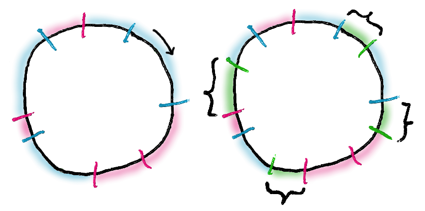
(cross-posted from the SwiftStack Blog)
In enabling mechanism to combine together general symbols, in successions of unlimited variety and extent, a uniting link is established between the operations of matter and the abstract mental processes of the most abstract branch of mathematical science. A new, a vast, and a powerful language is developed for the future use of analysis, in which to wield its truths so that these may become of more speedy and accurate practical application for the purposes of mankind [sic] than the means hitherto in our possession have rendered possible.
—Ada Lovelace on Charles Babbage's Analytical Engine, 1842
Dear reader, if you're reading [the SwiftStack Blog], you may have already heard that erasure codes have been added to OpenStack Swift (in beta for the 2.3.0 Kilo release, with continuing improvements thereafter) and that this is a really great thing that will make the world a better place.
All of this is entirely true. But what is perhaps less widely heard is exactly what erasure codes are and exactly why their arrival in Swift is a really great thing that will make the world a better place. That is what I aim to show you in this post—and I do mean show, not merely tell, for while integrating erasure codes into a production-grade storage system is (was!) an immense effort requiring months of work by some of the finest programmers the human race has to offer, the core idea is actually simple enough to fit in a (longish) blog post. Indeed, by the end of this post, we will have written a complete working implementation of a simple variant of Reed–Solomon coding, not entirely unlike what is used in Swift itself. No prior knowledge will be assumed except a working knowledge of high-school algebra and the Python programming language.
But first, we need to understand the problem that erasure codes solve. The strategy Swift has traditionally used to achieve its reliability and fault-tolerance properties is replication: keep more than one copy of each object (typically three), preferably in entirely different datacenters, failing that, on different machines, and failing that, at least on different hard drives. Your data is safe from occasional drive failures because the probability of all the drives containing a particular object failing at the same time is very, very small.
The problem with replication is that it's expensive: if you keep three replicas, then for every terabyte that you want to use, you have to pay for three terabytes of actual physical storage. The cost would appear to be unavoidable, unless ... unless there were some way to reap the benefits of distributing the information across different failure domains without storing the entire object at each location ...
"But surely this is impossible!" I hear you cry. "It's useless to make half a copy of something, because you can't know in advance of a disaster whether the half you made a backup of is the half that will need to be restored. In order to enjoy the safety of having a spare, you need a spare of the whole thing."
My dear reader, this objection is compelling, well-stated—and gloriously, one-hundred-percent wrong. We can achieve reliability guarantees similar to that of the replication strategy, keeping our data safe even as some of its fragments are damaged, lost, or erased. (Hence the name, erasure codes.) The method will have its own costs in the form of increased CPU load and more network requests; it won't make sense for all use cases, but when appropriate, the efficiency gain is impressive. It all depends on applying a deep philosophical insight into the nature of space itself.
Specifically: two points make a line.
Given any two distinct points on a plane, there is one and exactly one line that passes through both of them. We reconstruct anything we might want to know about a particular line just by remembering two points that it passes through.
But suppose we were to remember three points. Then we could still reconstruct the line from any two of them, which means that the information about our line hasn't been lost even if we forget one of the points.
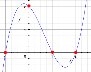
Similarly, three points make a parabola, four points make a cubic curve, and in full generality, m+1 points make a degree-m polynomial. Given n points on a polynomial curve where n is greater than m+1, any m+1 of them suffice to reconstruct the polynomial.
Thus, we have a clear strategy for storing data in a reliable, failure-tolerant way, without going to the expense of storing complete replicas: all we have to do is pretend our data is made out of polynomials, and store more points than are strictly necessary to reconstruct the data.
But don't take my word for it! Mere verbal arguments can be deceptive, but code is proof and code is truth, so if you still doubt that such an idea can really be made to work—and maybe you should—you won't after we're done implementing it.
So suppose we want to save some textual data; say, the string, "THE FUNDAMENTAL PROBLEM OF COMMUNICATION IS THAT OF REPRODUCING AT ONE POINT EITHER EXACTLY OR APPROXIMATELY A MESSAGE SELECTED AT ANOTHER POINT". Now, this data is made out of letters and spaces, not polynomials, but we can process it into a form that will make it easier to make-believe that it is. Say, we split the text into chunks of a fixed size (padding the end with extra spaces if necessary so that our chunk size evenly divides it), and convert the characters into integers from 0 to 26 (space is 0, A is 1, B is 2, &c.). Here are some functions to help with that—
from string import ascii_uppercase

ALPHABET = " "+ascii_uppercase
CHAR_TO_INT = dict(zip(ALPHABET, range(27)))
INT_TO_CHAR = dict(zip(range(27), ALPHABET))

def pad(text, chunk_size):
    return text + ' '*(chunk_size - len(text) % chunk_size)

def chunkify(text, chunk_size):
    return [text[i:i+chunk_size]
            for i in range(0, len(text), chunk_size)]

def convert(string):
    return [CHAR_TO_INT[c] for c in string]
After turning our text into converted chunks (lists of integers), we can interpret each chunk as representing the coefficients of a polynomial function: say, in order of increasing degree, so that, e.g., the list [1, 2, 3] represents the function \(1 + 2x + 3x^2\). Then we can take points on that polynomial at \(n\) different values of the independent variable \(x\) for some \(n\) greater than the chunk size to get a properly redundant encoding.
(It's actually better if you use polynomials over the finite field \(\mathbb{F}_q\) of the integers modulo \(q\) for some \(q\) which is a prime raised to the power of something, but let's not worry about that.)
def evaluate_polynomial(coefficients, x):
    return sum(c * x**i for i, c in enumerate(coefficients))

def encode(chunk, n):
    return [evaluate_polynomial(chunk, i) for i in range(n)]

def erasure_code(text, chunk_size, encoded_chunk_size):
    chunks = chunkify(pad(text, chunk_size), chunk_size)
    converted_chunks = [convert(chunk) for chunk in chunks]
    return [list(enumerate(encode(chunk, encoded_chunk_size)))
            for chunk in converted_chunks]
Then, with a choice for the original chunk size (which you'll recall will also be the number of terms each in the polynomials used to encode each chunk) and the size of the resulting encoded chunk (that is, the number of points we'll sample from the polynomials), we can encode our text.
$ python3
>>> from reed_solomon import *
>>> text = "THE FUNDAMENTAL PROBLEM OF COMMUNICATION IS THAT OF
REPRODUCING AT ONE POINT EITHER EXACTLY OR APPROXIMATELY A MESSAGE
SELECTED AT ANOTHER POINT"
>>> encoded = erasure_code(text, 5, 8)
>>> encoded
[[(0, 20), (1, 39), (2, 152), (3, 575), (4, 1668), (5, 3935), (6,
8024), (7, 14727)], [(0, 21), (1, 53), (2, 281), (3, 1179), (4, 3533),
(5, 8441), (6, 17313), (7, 31871)], [(0, 5), ...
[further output redacted]
At this point, our text has been transformed into a Python list, whose elements are Python lists representing the individual chunks, whose elements are tuples representing (x, y) coordinate pairs representing points on the polynomial representing that chunk.
Let's simulate distributing that encoded information across several storage nodes by writing points with different x-values to different files. We'll make-believe that each file is a different storage node. We'll write another function for that.
import json

def disperse(encoded_chunks):
    node_count = len(encoded_chunks[0])
    for i in range(node_count):
        with open('node'+str(i), 'w') as node:
            node.write(json.dumps([chunk[i] for chunk in encoded_chunks]))
And try it out—
>>> disperse(encoded)
>>>
$ ls
node0  node1  node2  node3  node4  node5  node6  node7
$ cat node4
[[4, 1668], [4, 3533], [4, 3517], [4, 1824], [4, 4080], [4, 4342],
[4, 1665], [4, 4769], [4, 5460], [4, 4172], [4, 4710], [4, 2254], [
4, 433], [4, 2436], [4, 4464], [4, 5796], [4, 1596], [4, 4428], [4,
 1417], [4, 5313], [4, 5452], [4, 709], [4, 6212], [4, 4973], [4, 5
445], [4, 5205], [4, 6308], [4, 4412], [4, 1555]]
In conclusion, that's how you use Reed–Solomon coding to turn comprehensible English text into inscrutable lists of lists of numbers distributed across several files. Thank you, and—
What's that you say, dear reader? Demonstrating how to encode something is useless unless you also demonstrate how to decode it? Well, I suppose you may have a point. Never fear—we can do that, too! But first, we'll need some functions for manipulating polynomials (in the "list of coefficients in order of ascending power" form that we've been using).
def get_coefficient(P, i):
    if 0 <= i < len(P):
        return P[i]
    else:
        return 0

def add_polynomials(P, Q):
    n = max(len(P), len(Q))
    return [get_coefficient(P, i) + get_coefficient(Q, i) for i in range(n)]

def scale_polynomial(P, a):
    return [a*c for c in P]

def multiply_polynomials(P, Q):
    maximum_terms = len(P) + len(Q)
    R = [0 for _ in range(maximum_terms)]
    for i, c in enumerate(P):
        for j, d in enumerate(Q):
            R[i+j] += c * d
    return R
Once we can do arithmetic with polynomials, we can write functions to reconstruct the polynomial representing a chunk of our text given our saved points, which is probably the most intricate part of this entire endeavor. We'll use a technical trick called Lagrange interpolation, after the great mathematician-astronomer Joseph-Louis Lagrange.
Suppose we want to reconstruct a cubic polynomial from the four points \((x_1, y_1)\), \((x_2, y_2)\), \((x_3, y_3)\), and \((x_4, y_4)\). It turns out that a formula for the polynomial is
$$y_1\ell_1(x) + y_2\ell_2(x) + y_3\ell_3(x) + y_4\ell_4(x)$$
where \(\ell_1(x)\) (the first Lagrange basis element) stands for
$$\frac{(x - x_2)(x - x_3)(x - x_4)}{(x_1 - x_2)(x_1 - x_3)(x_1 - x_4)}$$
and so on—for each \(i\) between 1 and the number of points we have, the numerator of the \(i\)th Lagrange basis element is the product of \((x - x_j)\) for all \(j\) from 1 up to the number of points we have but not equal to \(i\), and the denominator follows a similar pattern but with \(x_i\) instead of \(x\). (Note that we're using letters with subscripts, like \(x_i\), to represent specific constants, whereas \(x\) without a subscript is a function's independent variable.)
I hear you ask, "But why this particular arbitrary-looking formula out of the space of all possible arbitrary-looking formulae?" But the grace and beauty of this formula is exactly that it's engineered specifically to pass through our points. Consider what happens when we choose \(x\) equal to \(x_1\). The second through fourth terms \(y_2\ell_2(x_1)\) through \(y_4\ell_4(x_1)\) all contain a factor of \((x_1 - x_1)\) and are thus zero, but the first term becomes
$$y_1\frac{(x_1 - x_2)(x_1 - x_3)(x_1 - x_4)}{(x_1 - x_2)(x_1 - x_3)(x_1 - x_4)}$$
$$= y_1(1)$$
$$= y_1$$
So by design, our interpolated polynomial takes value \(y_1\) at \(x_1\), \(y_2\) at \(x_2\), and so forth. In Python, the whole process looks like this—
def lagrange_basis_denominator(xs, i):
    denominator = 1
    for j, x in enumerate(xs):
        if j == i:
            continue
        denominator *= xs[i] - xs[j]
    return denominator

def lagrange_basis_element(xs, i):
    element = [1]
    for j in range(len(xs)):
        if j == i:
            continue
        element = multiply_polynomials(element, [-xs[j], 1])
    scaling_factor = 1/lagrange_basis_denominator(xs, i)
    return scale_polynomial(element, scaling_factor)

def interpolate(points):
    result = [0]
    xs, ys = zip(*points)
    for i in range(len(points)):
        result = add_polynomials(
            result,
            scale_polynomial(lagrange_basis_element(xs, i), ys[i])
        )
    return [round(k) for k in result]
(Note that we're rounding off our computed coefficients because this implementation isn't very numerically stable—the subtle differences between true real-number arithmetic and the approximate floating-point arithmetic implemented by computers start to accumulate, and if we choose too large of a chunk size, our program will actually start giving the wrong answers—but let's not worry about that, either.)
With this technique, we now have all the tools we need to recover our text from a subset of the data we wrote to our various "nodes" earlier. What we need to do is this: for each chunk, arbitrarily select a number of stored points equal to our chunk size, interpolate the polynomial from them, deconvert the numbers which are the coefficients of that polynomial back into their character equivalents, unchunkify the chunks into a unified whole, and unpad any whitespace we added to the end when we began.
def deconvert(sequence):
    return ''.join(INT_TO_CHAR[i] for i in sequence)

def unchunkify(chunks):
    return ''.join(chunks)

def unpad(text):
    return text.rstrip()

def erasure_decode(encoded_chunks, chunk_size, encoded_chunk_size):
    converted_chunks = [interpolate(chunk[:chunk_size])[:chunk_size]
                        for chunk in encoded_chunks]
    return unpad(unchunkify(deconvert(chunk) for chunk in converted_chunks))
But about that data that we wrote out earlier.
$ ls
node0  node1  node2  node3  node4  node5  node6  node7
It would hardly be a compelling test of our erasure-coding skills if there were any suspicion that we actually needed all of those files—we really only need as many as our chunk size. So let's suppose that three of our nodes die in a fire—
$ rm node1 node3 node6
$ ls
node0  node2  node4  node5  node7
Could this the end of our data? With a full three-eighths of our encoding having been utterly destroyed, is it delusional to hold out hope that our text might yet be faithfully recovered? No! No, it is not! We only need one more function to retrieve the encoded chunks—
def retrieve(*nodes):
    responses = []
    for node in nodes:
        with open(node) as our_node:
            responses.append(json.loads(our_node.read()))
    return [[response[i] for response in responses]
            for i in range(len(responses[0]))]
—and then—
$ python3
>>> from reed_solomon import *
>>> node_data = retrieve("node0", "node2", "node4", "node5", "node7")
—successfully decode them!
>>> erasure_decode(node_data, 5, 8)
'THE FUNDAMENTAL PROBLEM OF COMMUNICATION IS THAT OF REPRODUCING AT
 ONE POINT EITHER EXACTLY OR APPROXIMATELY A MESSAGE SELECTED AT AN
OTHER POINT'
Dear reader, it is true our toy implementation here was crude, the hundred-and-change bytes of data we demonstrated it on was of no intrinsic interest, and many obvious and not-so-obvious subtleties were ignored. But I implore you to consider the implications for your own storage needs of more advanced, not-merely-educational application of these vast and powerful techniques. Imagine just how soundly you'll be able to sleep at night knowing that you're well under your budget and yet your data is just as safe as if you had three complete independent copies of it!
And even if you personally have no intention of deploying Swift—as my SwiftStack colleague and project technical lead for OpenStack Swift John Dickinson has pointed out, we are rapidly entering an era in which everyone uses object storage, whether they realize it or not. In a hyperconnected global economy, even minor efficiency improvements in key infrastructure components can reap enormous benefits elsewhere, which is to say that the rest of your life will contain more happiness and less pain if the financial institution that invests your retirement savings, or the medical research institute that develops a cure for the cancer you'll get twenty years from now, or the image hosting service that serves you cute cat pictures today, have access to cheaper, faster, and more reliable storage than the means hitherto in our possession have rendered possible. And that's why erasure codes being in OpenStack Swift is a really great thing that will make the world a better place; quod erat demonstrandum.
The code in this post is available separately.