An Algorithmic Lucidity

(originally published at Less Wrong)

As a casual formal epistemology fan, you've probably heard that the philosophical notion of causality can be formalized in terms of Bayesian networks—but also as a casual formal epistemology fan, you also probably don't know the details all that well.

One day, while going through the family archives, you come across a meticulously maintained dataset describing a joint probability distribution over four variables: whether it rained that day, whether the sprinkler was on, whether the sidewalk was wet, and whether the sidewalk was slippery. The distribution is specified in this table (using the abbreviated labels "rain", "slippery", "sprinkler", and "wet"):

(You wonder what happened that one day out of 140,000 when it rained, and the sprinkler was on, and the sidewalk was slippery but not wet. Did—did someone put a tarp up to keep the sidewalk dry, but also spill slippery oil, which didn't count as being relevantly "wet"? Also, 140,000 days is more than 383 years—were "sprinklers" even a thing in the year 1640 C.E.? You quickly put these questions out of your mind: it is not your place to question the correctness of the family archives.)

You're slightly uncomfortable with this unwieldy sixteen-row table. You think that there must be some other way to represent the same information, while making it clearer that it's not a coincidence that rain and wet sidewalks tend to co-occur.

You've read that Bayesian networks "factorize" an unwieldly joint probability distribution into a number of more compact conditional probability distributions, related by a directed acyclic graph, where the arrows point from "cause" to "effect". (Even a casual formal epistemology fan knows that much.) The graph represents knowledge that each variable is conditionally independent of its non-descendants given its parents, which enables "local" computations: given the values of just a variable's parents in the graph, we can compute a conditional distribution for that variable, without needing to consider what is known about other variables elsewhere in the graph ...

You've read that, but you've never actually done it before! You decide that constructing a Bayesian network to represent this distribution will be a useful exercise.

To start, you re-label the variables for brevity. (On a whim, you assign indices in reverse-alphabetical order: \(X_1\) = wet, \(X_2\) = sprinkler, \(X_3\) = slippery, \(X_4\) = rain.)

Now, how do you go about building a Bayesian network? As a casual formal epistemology fan, you are proud to own a copy of the book by Daphne Koller and the other guy, which explains how to do this in—you leaf through the pages—probably §3.4, "From Distributions to Graphs"?—looks like ... here, in Algorithm 3.2. It says to start with an empty graph, and it talks about random variables, and setting directed edges in the graph, and you know from chapter 2 that the ⟂ and | characters are used to indicate conditional independence. That has to be it.

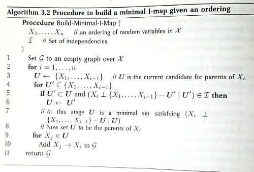
(As a casual formal epistemology fan, you haven't actually read chapter 3 up through §3.4, but you don't see why that would be necessary, since this Algorithm 3.2 pseudocode is telling you what you need to do.)

It looks like the algorithm says to pick a variable, allocate a graph node to represent it, find the smallest subset of the previously-allocated variables such that the variable represented by the new node is conditionally independent of the other previously-allocated variables given that subset, and then draw directed edges from each of the nodes in the subset to the new node?—and keep doing that for each variable—and then compute conditional probability tables for each variable given its parents in the resulting graph?

That seems complicated when you say it abstractly, but you have faith that it will make more sense as you carry out the computations.

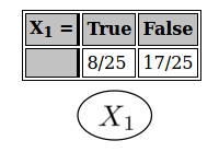
First, you allocate a graph node for \(X_1\). It doesn't have any parents, so the associated conditional ("conditional") probability distribution, is really just the marginal distribution for \(X_1\).

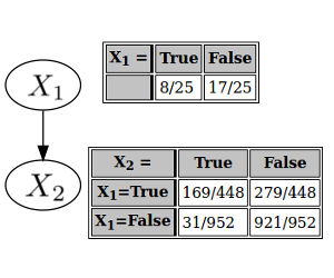
Then you allocate a node for \(X_2\). \(X_2\) is not independent of \(X_1\). (Because \(P(X_1 \land X_2)\) = 169/1400, which isn't the same as \(P(X_1) \cdot P(X_2)\) = 8/25 · 1/7 = 8/175.) So you make \(X_1\) a parent of \(X_2\), and your conditional probability table for \(X_2\) separately specifies the probabilities of \(X_2\) being true or false, depending on whether \(X_1\) is true or false.

Next is \(X_3\). Now that you have two possible parents, you need to check whether conditioning on either of \(X_1\) and \(X_2\) would render \(X_3\) conditionally independent of the other. If not, then both \(X_1\) and \(X_2\) will be parents of \(X_3\); if so, then the variable you conditioned on will be the sole parent. (You assume that the case where \(X_3\) is just independent from both \(X_1\) and \(X_2\) does not pertain; if that were true, \(X_3\) wouldn't be connected to the rest of the graph at all.)

It turns out that \(X_3\) and \(X_2\) are conditionally independent given \(X_1\). That is, \(P(X_3 \land X_2 \mid X_1) = P(X_3 \mid X_1) \cdot P(X_2 \mid X_1)\). (Because the left-hand side is \(\frac{P(X_3 \land X_2 \land X_1)}{P(X_1)} = \frac{507}{1792}\), and the right-hand side is \(\frac{3}{4} \cdot \frac{169}{448} = \frac{507}{1792}\).) So \(X_1\) is a parent of \(X_3\), and \(X_2\) isn't; you draw an arrow from \(X_1\) (and only \(X_1\)) to \(X_3\), and compile the corresponding conditional probability table.

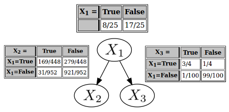
Finally, you have \(X_4\). The chore of finding the parents is starting to feel more intuitive now. Out of the \(2^3 = 8\) possible subsets of the preceding variables, you need to find the smallest subset, such that conditioning on that subset renders \(X_4\) (conditionally) independent of the variables not in that subset. After some calculations that the authors of expository blog posts have sometimes been known to callously leave as an exercise to the reader, you determine that \(X_1\) and \(X_2\) are the parents of \(X_4\).

And with one more conditional probability table, your Bayesian network is complete!

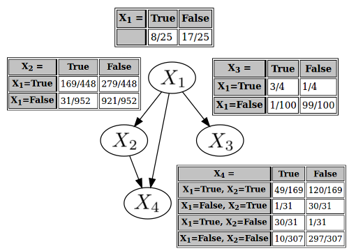
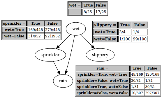
Eager to interpret the meaning of this structure regarding the philosophy of causality, you translate the \(X_i\) variable labels back to English:

...

This can't be right. The arrow from "wet" to "slippery" seems fine. But all the others are clearly absurd. Wet sidewalks cause rain? Sprinklers cause rain? Wet sidewalks cause the sprinkler to be on?

You despair. You thought you had understood the algorithm. You can't find any errors in your calculations—but surely there must be some? What did you do wrong?

After some thought, it becomes clear that it wasn't just a calculation error: the procedure you were trying to carry out couldn't have given you the result you expected, because it never draws arrows from later-considered to earlier-considered variables. You considered "wet" first. You considered "rain" last, and then did independence tests to decide whether or not to draw arrows from "wet" (or "sprinkler" or "slippery") to "rain". An arrow from "rain" to "wet" was never a possibility. The output of the algorithm is sensitive to the ordering of the variables.

(In retrospect, that probably explains the "given an ordering" part of Algorithm 3.2's title, "Procedure to build a minimal I-map given an ordering." You hadn't read up through the part of chapter 3 that presumably explains what an "I-map" is, and had disregarded the title as probably unimportant.)

You try carrying out the algorithm with the ordering "rain", "sprinkler", "wet", "slippery" (or \(X_4\), \(X_2\), \(X_1\), \(X_3\) using your \(X_i\) labels from before), and get this network:

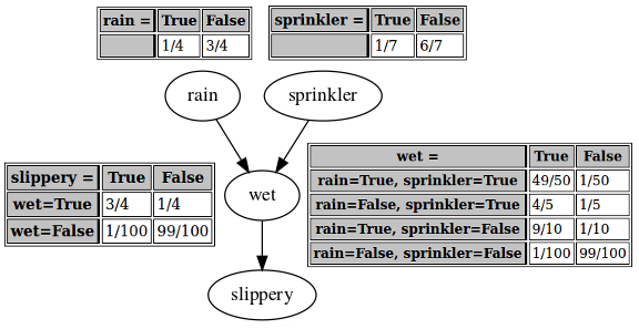
—for which giving the arrows a causal interpretation seems much more reasonable.

You notice that you are very confused. The "crazy" network you originally derived, and this "true" network derived from a more intuitively causal variable ordering, are different: they don't have the same structure, and (except for the wet → slippery link) they don't have the same conditional probability tables. You would assume that they can't "both be right". If the network output by the algorithm depends on what variable ordering you use, how are you supposed to know which ordering is correct? In this example, you know from reasons outside the math, that "wet" shouldn't cause "rain", but you couldn't count on that were you to apply these methods to problems further removed from intuition.

Playing with both networks, you discover that despite their different appearances, they both seem to give the same results when you use them to calculate marginal or conditional probabilities. For example, in the "true" network, \(P(\mathrm{rain})\) is 1/4 (read directly from the "conditional" probability table, as "rain" has no parents in the graph). In the "crazy" network, the probability of rain can be computed as

... which also equals 1/4.

That actually makes sense. You were wrong to suppose that the two networks couldn't "both be right". They are both right; they both represent the same joint distribution. The result of the algorithm for constructing a Bayesian network—or a "minimal I-map", whatever that is—depends on the given variable ordering, but since the algorithm is valid, each of the different possible results is also valid.

But if the "crazy" network and the "true" network are both right, what happened to the promise of understanding causality using Bayesian networks?! (You may only be a casual formal epistemology fan, but you remember reading a variety of secondary sources unanimously agreeing that this was a thing; you're definitely not misremembering or making it up.) If both networks give the same answers to marginal and conditional probability queries, that amounts to them making the same predictions about the world. So if beliefs are supposed to correspond to predictions, in what sense could the "true" network be better? What does your conviction that rain causes wetness even mean, if someone who believed the opposite could make all the same predictions?

You remember the secondary sources talking about interventions on causal graphs: severing a node from its parents and forcing it to take a particular value. And the "crazy" network and the "true" network do differ with respect to that operation: in the "true" network, setting "wet" to be false—you again imagine putting a tarp up over the sidewalk—wouldn't change the probability of "rain". But in the "crazy" network, forcing "wet" to be false would change the probability of rain—to \(P(\mathrm{rain} \mid \mathrm{sprinkler}, \neg \mathrm{wet}) \cdot P(\mathrm{sprinkler} \mid \neg \mathrm{wet}) + P(\mathrm{rain} \mid \neg \mathrm{sprinkler}, \neg \mathrm{wet}) \cdot P(\neg \mathrm{sprinkler} \mid \neg \mathrm{wet})\), which is \(\frac{1}{31} \cdot \frac{31}{952} + \frac{10}{307} \cdot \frac{921}{952} \approx 0.032\) (greatly reduced from the 1/4 you calculated a moment ago). Notably, this intervention—\(P(\mathrm{rain} \mid \mathrm{do}(\neg \mathrm{wet}))\), if you're remembering correctly what some of the secondary sources said about a do operator—isn't the same thing as the conditional probability \(P(\mathrm{rain}| \neg \mathrm{wet})\).

This would seem to satisfy your need for a sense in which the "true" network is "better" than the "crazy" network, even if Algorithm 3.2 indifferently produces either depending on the ordering it was given. (You're sure that Daphne Koller and the other guy have more to say about other algorithms that can make finer distinctions, but this feels like enough studying for one day—and enough for one expository blog post, if someone was writing one about your inquiries. You're a casual formal epistemology fan.) The two networks represent the same predictions about the world recorded in your family archives, but starkly different predictions about nearby possible worlds—about what would happen if some of the factors underlying the world were to change.

You feel a slight philosophical discomfort about this. You don't like the idea of forced change, of intervention, being so integral to such a seemingly basic notion as causality. It feels almost anthropomorphic: you want the notion of cause and effect within a system to make sense without reference to the intervention of some outside agent—for there's nothing outside of the universe. But whether this intuition is a clue towards deeper insights, or just a place where your brain has tripped on itself and gotten confused, it's more than you understand now.

(originally published at Less Wrong)

There's this statistical phenomenon where it's possible for two multivariate distributions to overlap along any one variable, but be cleanly separable when you look at the entire configuration space at once. This is perhaps easiest to see with an illustrative diagram—

The denial of this possibility (in arguments of the form, "the distributions overlap along this variable, therefore you can't say that they're different") is sometimes called the "univariate fallacy." (Eliezer Yudkowsky proposes "covariance denial fallacy" or "cluster erasure fallacy" as potential alternative names.)

Let's make this more concrete by making up an example with actual numbers instead of just a pretty diagram. Imagine we have some datapoints that live in the forty-dimensional space {1, 2, 3, 4}⁴⁰ that are sampled from one of two probability distibutions, which we'll call \(P_A\) and \(P_B\).

For simplicity, let's suppose that the individual variables x₁, x₂, ... x₄₀—the coördinates of a point in our forty-dimensional space—are statistically independent. For every individual \(x_i\), the marginal distribution of \(P_A\) is—

And for \(P_B\)—

If you look at any one \(x_i\)-coördinate for a point, you can't be confident which distribution the point was sampled from. For example, seeing that x₁ takes the value 2 gives you a 7/4 (= 1.75) likelihood ratio in favor of that the point having been sampled from \(P_A\) rather than \(P_B\), which is log₂(7/4) ≈ 0.807 bits of evidence.

That's ... not a whole lot of evidence. If you guessed that the datapoint came from \(P_A\) based on that much evidence, you'd be wrong about 4 times out of 10. (Given equal (1:1) prior odds, an odds ratio of 7:4 amounts to a probability of (7/4)/(1 + 7/4) ≈ 0.636.)

And yet if we look at many variables, we can achieve supreme, godlike confidence about which distribution a point was sampled from. Proving this is left as an exercise to the particularly intrepid reader, but a concrete demonstration is probably simpler and should be pretty convincing! Let's write some Python code to sample a point x⃗ ∈ {1, 2, 3, 4}⁴⁰ from \(P_A\)—

import random

def a():
    return random.sample(
        [1]*4 +  # 1/4
        [2]*7 +  # 7/16
        [3]*4 +  # 1/4
        [4],     # 1/16
        1
    )[0]

x = [a() for _ in range(40)]
print(x)

Go ahead and run the code yourself. (With an online REPL if you don't have Python installed locally.) You'll probably get a value of x that "looks something like"

[2, 1, 2, 2, 1, 1, 2, 2, 1, 2, 1, 4, 4, 2, 2, 3, 3, 1, 2, 2, 2, 4, 2, 2, 1, 2, 1, 4, 3, 3, 2, 1, 1, 3, 3, 2, 2, 3, 3, 4]

If someone off the street just handed you this x⃗ without telling you whether she got it from \(P_A\) or \(P_B\), how would you compute the probability that it came from \(P_A\)?

Well, because the coördinates/variables are statistically independent, you can just tally up (multiply) the individual likelihood ratios from each variable. That's only a little bit more code—

import logging

logging.basicConfig(level=logging.INFO)

def odds_to_probability(o):
    return o/(1+o)

def tally_likelihoods(x, p_a, p_b):
    total_odds = 1
    for i, x_i in enumerate(x, start=1):
        lr = p_a[x_i-1]/p_b[x_i-1]  # (-1s because of zero-based array indexing)
        logging.info("x_%s = %s, likelihood ratio is %s", i, x_i, lr)
        total_odds *= lr
    return total_odds

print(
    odds_to_probability(
        tally_likelihoods(
            x,
            [1/4, 7/16, 1/4, 1/16],
            [1/16, 1/4, 7/16, 1/4]
        )
    )
)

If you run that code, you'll probably see "something like" this—

INFO:root:x_1 = 2, likelihood ratio is 1.75
INFO:root:x_2 = 1, likelihood ratio is 4.0
INFO:root:x_3 = 2, likelihood ratio is 1.75
INFO:root:x_4 = 2, likelihood ratio is 1.75
INFO:root:x_5 = 1, likelihood ratio is 4.0
[blah blah, redacting some lines to save vertical space in the blog post, blah blah]
INFO:root:x_37 = 2, likelihood ratio is 1.75
INFO:root:x_38 = 3, likelihood ratio is 0.5714285714285714
INFO:root:x_39 = 3, likelihood ratio is 0.5714285714285714
INFO:root:x_40 = 4, likelihood ratio is 0.25
0.9999936561215961

Our computed probability that x⃗ came from \(P_A\) has several nines in it. Wow! That's pretty confident!

Thanks for reading!