An Algorithmic Lucidity

(originally published at Less Wrong)

Sometimes, people are reluctant to admit that they were wrong about something, because they're afraid that "You are wrong about this" carries inextricable connotations of "You are stupid and bad." But this behavior is, itself, wrong, for at least two reasons.

First, because it's evidential decision theory. The so-called "rationalist" "community" has a lot of cached clichés about this! A blank map does not correspond to a blank territory. What's true is already so; owning up to it doesn't make it worse. Refusing to go to the doctor (thereby avoiding encountering evidence that you're sick) doesn't keep you healthy.

If being wrong means that you're stupid and bad, then preventing yourself from knowing that you were wrong doesn't stop you from being stupid and bad in reality. It just prevents you from knowing that you're stupid and bad—which is an important fact to know (if it's true), because if you don't know that you're stupid and bad, then it probably won't occur to you to even look for possible interventions to make yourself less stupid and less bad.

Second, while "You are wrong about this" is evidence for the "You are stupid and bad" hypothesis if stupid and bad people are more likely to be wrong, I claim that it's very weak evidence. (Although it's possible that I'm wrong about this—and if I'm wrong, it's furthermore possible that the reason I'm wrong is because I'm stupid and bad.)

Exactly how weak evidence is it? It's hard to guess directly, but fortunately, we can use probability theory to reduce the claim into more "atomic" conditional and prior probabilities that might be easier to estimate!

Let \(W\) represent the proposition "You are wrong about something", \(S\) represent the proposition "You are stupid", and \(B\) represent the proposition "You are bad."

By Bayes's theorem, the probability that you are stupid and bad given that you're wrong about something is given by—

For the purposes of this calculation, let's assume that badness and stupidity are statistically independent. I doubt this is true in the real world, but because I'm stupid and bad (at math), I want that simplifying assumption to make the algebra easier for me. That lets us unpack the conjunctions, giving us—

This expression has six degrees of freedom: \(P(S)\), \(P(B)\), \(P(W|S,B)\), \(P(W|S, \neg B)\), \(P(W|\neg S,B)\), \(P(W|\neg S, \neg B)\). Arguing about the values of these six individual parameters is probably more productive than arguing about the value of \(P(S,B|W)\) directly!

Suppose half the people are stupid (\(P(S) = 0.5\)), one-tenth of people are bad (\(P(B) = 0.1\)), and that most people are wrong, but that being stupid or bad each make you somewhat more likely to be wrong, to the tune of \(P(W|\neg S, \neg B) = 0.8\), \(P(W|S, \neg B) = P(W|\neg S,B) = 0.85\), and \(P(W|S,B) = 0.9\). So our posterior probabilty that someone is stupid and bad given that they were wrong once is

But the base rate of being stupid and bad is (0.1)(0.5) = 0.05. Learning that someone was wrong only raised our probability that they are stupid and bad by 0.0042. That's a small number that you shouldn't worry about!

"The sink is full and it's your turn to do the dishes! Ugh, why are you so inconsiderate of others?!"

"Not true! Note that the dishes pile up just as badly when you're away."

"So?"

"So, it's not that I'm inconsiderate of others; I'm inconsiderate towards people in the future, independently of whether they happen to be me."

(originally published at Less Wrong)

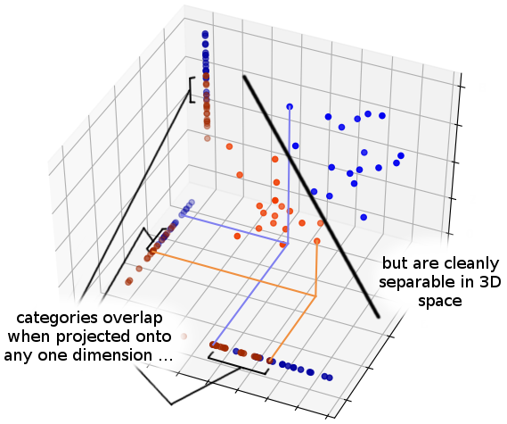
There's this statistical phenomenon where it's possible for two multivariate distributions to overlap along any one variable, but be cleanly separable when you look at the entire configuration space at once. This is perhaps easiest to see with an illustrative diagram—

The denial of this possibility (in arguments of the form, "the distributions overlap along this variable, therefore you can't say that they're different") is sometimes called the "univariate fallacy." (Eliezer Yudkowsky proposes "covariance denial fallacy" or "cluster erasure fallacy" as potential alternative names.)

Let's make this more concrete by making up an example with actual numbers instead of just a pretty diagram. Imagine we have some datapoints that live in the forty-dimensional space {1, 2, 3, 4}⁴⁰ that are sampled from one of two probability distibutions, which we'll call \(P_A\) and \(P_B\).

For simplicity, let's suppose that the individual variables x₁, x₂, ... x₄₀—the coördinates of a point in our forty-dimensional space—are statistically independent. For every individual \(x_i\), the marginal distribution of \(P_A\) is—

And for \(P_B\)—

If you look at any one \(x_i\)-coördinate for a point, you can't be confident which distribution the point was sampled from. For example, seeing that x₁ takes the value 2 gives you a 7/4 (= 1.75) likelihood ratio in favor of that the point having been sampled from \(P_A\) rather than \(P_B\), which is log₂(7/4) ≈ 0.807 bits of evidence.

That's ... not a whole lot of evidence. If you guessed that the datapoint came from \(P_A\) based on that much evidence, you'd be wrong about 4 times out of 10. (Given equal (1:1) prior odds, an odds ratio of 7:4 amounts to a probability of (7/4)/(1 + 7/4) ≈ 0.636.)

And yet if we look at many variables, we can achieve supreme, godlike confidence about which distribution a point was sampled from. Proving this is left as an exercise to the particularly intrepid reader, but a concrete demonstration is probably simpler and should be pretty convincing! Let's write some Python code to sample a point x⃗ ∈ {1, 2, 3, 4}⁴⁰ from \(P_A\)—

import random

def a():
    return random.sample(
        [1]*4 +  # 1/4
        [2]*7 +  # 7/16
        [3]*4 +  # 1/4
        [4],     # 1/16
        1
    )[0]

x = [a() for _ in range(40)]
print(x)

Go ahead and run the code yourself. (With an online REPL if you don't have Python installed locally.) You'll probably get a value of x that "looks something like"

[2, 1, 2, 2, 1, 1, 2, 2, 1, 2, 1, 4, 4, 2, 2, 3, 3, 1, 2, 2, 2, 4, 2, 2, 1, 2, 1, 4, 3, 3, 2, 1, 1, 3, 3, 2, 2, 3, 3, 4]

If someone off the street just handed you this x⃗ without telling you whether she got it from \(P_A\) or \(P_B\), how would you compute the probability that it came from \(P_A\)?

Well, because the coördinates/variables are statistically independent, you can just tally up (multiply) the individual likelihood ratios from each variable. That's only a little bit more code—

import logging

logging.basicConfig(level=logging.INFO)

def odds_to_probability(o):
    return o/(1+o)

def tally_likelihoods(x, p_a, p_b):
    total_odds = 1
    for i, x_i in enumerate(x, start=1):
        lr = p_a[x_i-1]/p_b[x_i-1]  # (-1s because of zero-based array indexing)
        logging.info("x_%s = %s, likelihood ratio is %s", i, x_i, lr)
        total_odds *= lr
    return total_odds

print(
    odds_to_probability(
        tally_likelihoods(
            x,
            [1/4, 7/16, 1/4, 1/16],
            [1/16, 1/4, 7/16, 1/4]
        )
    )
)

If you run that code, you'll probably see "something like" this—

INFO:root:x_1 = 2, likelihood ratio is 1.75
INFO:root:x_2 = 1, likelihood ratio is 4.0
INFO:root:x_3 = 2, likelihood ratio is 1.75
INFO:root:x_4 = 2, likelihood ratio is 1.75
INFO:root:x_5 = 1, likelihood ratio is 4.0
[blah blah, redacting some lines to save vertical space in the blog post, blah blah]
INFO:root:x_37 = 2, likelihood ratio is 1.75
INFO:root:x_38 = 3, likelihood ratio is 0.5714285714285714
INFO:root:x_39 = 3, likelihood ratio is 0.5714285714285714
INFO:root:x_40 = 4, likelihood ratio is 0.25
0.9999936561215961

Our computed probability that x⃗ came from \(P_A\) has several nines in it. Wow! That's pretty confident!

Thanks for reading!